Introduction

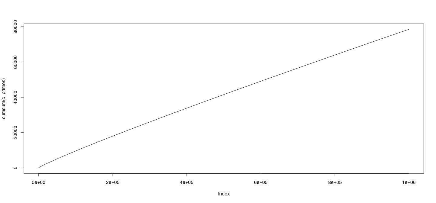
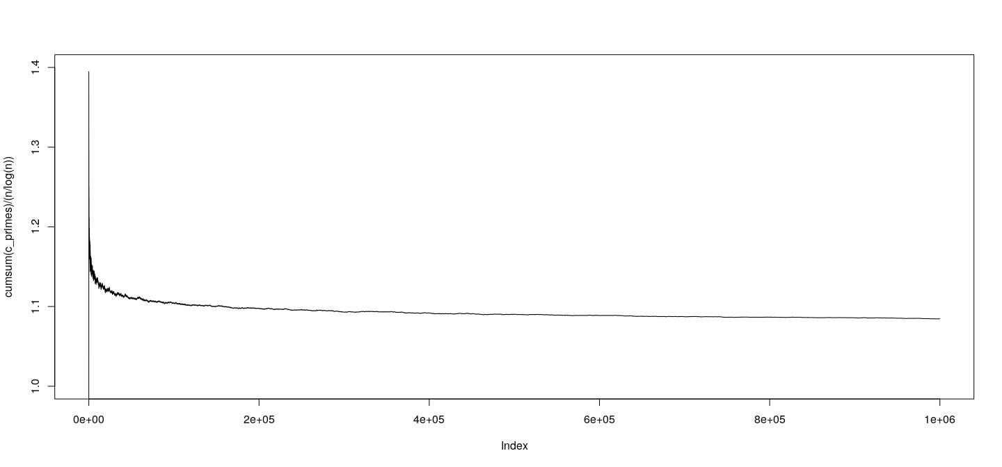
# Introduction - 2

## Introductory Computer Programming

### Deepayan Sarkar

---

# Functions and control flow structures

---

* The main components of our programs are going to be functions

* Functions usually

- have one or more input arguments,

- perform some computations, possibly calling other functions, and

- return one or more output values.

* The second step is the main contribution of a function
--

* Usually a programming language will already have many built-in functions

* These can be called by other functions

* Knowing what is available is an essential part of "learning" a language

---

* The standard model for performing computations is __sequential
  execution__

* In other words, a function executes a set of instructions in a specified sequence

* Some control flow structures may be used to create branches or loops
  in the flow of execution
  
---

* Briefly, the main ingredients used are

- Declaration of variables (implicit in some languages)

- Evaluation of expressions. _Can involve variables provided they
	  have been defined in an earlier step_

- Assignment to variables (to store intermediate results for later use)

- Logical tests (equal?, less than?, greater than?, is more input available?)

- Logical operations (AND, OR, NOT, XOR)

- Branching - take different paths based on result of a logical
	  operation (if-then-else)

- Loops - repeat sequence of steps, a fixed number of times, or
	  while a condition holds (for / while)
--

* The details of how variables store values, and who can access them
  (scope) are important
  
* But we will not worry about these issues for now

---

# Common operators (may have language-specific variants)

- _Mathematical operators_: 
    - `+` (addition)
	- `*` (multiplication)
	- `/` (division --- possibly integer division)
	- `^` (power)
	- `%` (the modulo operation)

- _Logical operators_: 
	- `&` (AND)
	- `|` (OR)
	- `!` (NOT)

- _Comparisons_: 
	- `==` (equality)
	- `!=` ($\neq$)
	- `<`, `>` (strictly less than or greater than) 
	- `<=` `>=` ($\leq$, $\geq$)

- _Mathematical functions_: `round, floor, ceil, abs, sqrt, exp, log, sin, cos, ...`

---

# Practical implementation: programming languages

* The algorithms we discuss can be implemented in many programming languages

* Some standard languages suitable for structured programming are

- [C](https://en.wikipedia.org/wiki/C_%28programming_language%29) (compiled)
	- [C++](https://en.wikipedia.org/wiki/C_%28programming_language%29) (compiled)
	- [R](https://en.wikipedia.org/wiki/R_%28programming_language%29) (interpreted)
	- [Python](https://en.wikipedia.org/wiki/Python_%28programming_language%29) (interpreted)
	- [Julia](https://en.wikipedia.org/wiki/Julia_%28programming_language%29) (interpreted)

* There are also many others with various relative strengths and weaknesses

* In this course, we will mainly focus on

- __R__ because it already has an extensive collection of statistical tools that we can use

- __C__ / __C++__ because it is easy to call C / C++ code from R (useful when R code is inefficient)

---

# Example: The `is_prime` algorithm in various languages

* Recall the `is_prime` algorithm to determine if a number is prime

* With slight modification to use only integer arithmetic

.algorithm[
.name[`is\_prime(n)`]
i := 2
__while__ (i * i $\leq$ n) {
    __if__ (n mod i == 0) {
        __return__ FALSE
    }
  i := i + 1
}
__return__ TRUE
]

---

# Example: The `is_prime` algorithm in various languages

* Implemented in C, the algorithm would look like this:

```c
int is_prime_c(int n) 
{
	int i = 2;
	while (i * i <= n) {
		if (n % i == 0) {
			return 0;
		}
		i = i + 1;
	}
	return 1;
}
```

* C is a compiled language, so actually running this code involves
  some additional work

* Note that all variable _types_ need to be explicitly declared

* This includes the types of function arguments (inputs) and return value (output)

---

# Example: The `is_prime` algorithm in various languages

* The same algorithm would look like this in R:

```r
is_prime_r <- function(n)
{
	i <- 2
	while (i * i <= n) {
		if (n %% i == 0) {
			return (FALSE)
		}
		i <- i + 1
	}
	return (TRUE)
}
```

* The basic structure is very similar, but with some differences:

- The assignment operator is different (but `=` also works in R)
    - The function declaration looks like a variable assignment
    - The modulo operator is `%%` instead of `%`
    - Uses `TRUE` and `FALSE` instead of `1` and `0` for logical values
	- Statements do not end with a semicolon (although they could)
	- Variable types are not declared
	- The return value must be put in parentheses

---

# Example: The `is_prime` algorithm in various languages

* We can call this function after starting R and copy-pasting the function definition

```r
is_prime_r(4)
```

```
[1] FALSE
```

```r
is_prime_r(10)
```

```
[1] FALSE
```

```r
is_prime_r(100)
```

```
[1] FALSE
```

```r
is_prime_r(101)
```

```
[1] TRUE
```

---

# Example: The `is_prime` algorithm in various languages

* The implementation looks a little different in Python:

```python
def is_prime_py(n):
	i = 2
	while i * i <= n:
		if n % i == 0:
			return 0;
		i = i + 1
	return 1
```

* The main difference is in how code blocks are defined:

- start with a colon (`:`) 
	
	- end is defined by indentation (amount of space in the beginning)

* Changing indentation will change meaning of code, which does not happen in C or R

* However, code in all languages _should be indented properly for readability_

---

# Example: The `is_prime` algorithm in various languages

* Again, we can start python, define the function, and run the following code

```python
print(is_prime_py(4))
```

```
0
```

```python
print(is_prime_py(10))
```

```
0
```

```python
print(is_prime_py(100))
```

```
0
```

```python
print(is_prime_py(101))
```

```
1
```

---

# How can we run C / C++ code?

---

* The code needs to be "compiled" before it is run

* It also needs a `main()` function to be defined

* `main()` is run first when the program is executed

* Here is a [complete file](cdemo/is_prime_wrapper.c) that can be compiled

---

```c
#include <stdio.h>
#include <stdlib.h>

int is_prime_c(int n) 
{
    int i = 2;
    while (i * i <= n) {
		if (n % i == 0) {
			return 0;
		}
		i = i + 1;
    }
    return 1;
}

int main(int argc, char *argv[])
{
    int i, n;
    if (argc > 1) {    /* one or more arguments supplied  */
		for (i = 1; i < argc; i++) {
			n = atoi(argv[i]); 	/* converts string to integer */
			printf("%d -> %d\n", n, is_prime_c(n));
		}
    }
    else printf("Usage: %s <n1> <n2> ...\n", argv[0]);
    return 0;
}
```

---

* How to compile & run depends on the operating system

* For example, on Linux / Mac, something like the following should work

```bash
gcc -o is_prime cdemo/is_prime_wrapper.c
./is_prime
```

```
Usage: ./is_prime <n1> <n2> ...
```

```bash
./is_prime  4 10 100 101
```

```
4 -> 0
10 -> 0
100 -> 0
101 -> 1
```

---

# Compiled code vs interpreted code

* R, Python, etc., are "interpreted" languages that read and evaluate code interactively

* Compiled code is usually (but not always) much faster than interpreters

* Most interpreters are themselves written in a compiled language

* However, compiled languages have several disadvantages:

* They are not interactive!

* Trying out ideas (edit-compile-run) takes longer

* Most importantly: limited initial set of tools

* For example, you will need to write your own functions to import data, make plots, etc.

* Ultimately, choice depends on the purpose of the program

---

# Compiled code vs interpreted code

* We will mainly use R (to take advantage of its many useful features)

* We will not write C programs designed to be run directly

* However, we _will_ sometimes call C / C++ code __from R__ to take advantage of its speed

* The easiest way to do this is using a _package_ called [Rcpp](https://cran.r-project.org/package=Rcpp)

* Python code can similarly be called using the [reticulate](https://cran.r-project.org/package=reticulate) package

* And Julia code can be called using the [JuliaCall](https://cran.r-project.org/package=JuliaCall) package

* I will give an example of Rcpp to illustrate its usefulness

* We will look at it in more detail after learning more about R and C

---

# An example of using Rcpp

* The first step is to compile a C function so that it can be called from R

```r
library(package = "Rcpp")
sourceCpp(code = 
"

#include <Rcpp.h>

// [[Rcpp::export]]
int is_prime_c(int n) 
{
	int i = 2;
	while (i * i <= n) {
		if (n % i == 0) {
			return 0;
		}
		i = i + 1;
	}
	return 1;
}

")
```

---

# An example of using Rcpp

* Alternatively, compile code in a [file](cdemo/is_prime_rcpp.cpp)

```r
library(package = "Rcpp")
sourceCpp("cdemo/is_prime_rcpp.cpp")
```

---

# An example of using Rcpp

* The C function can then be called just like an R function

```r
is_prime_c(4)
```

```
[1] 0
```

```r
is_prime_c(10)
```

```
[1] 0
```

```r
is_prime_c(100)
```

```
[1] 0
```

```r
is_prime_c(101)
```

```
[1] 1
```

---

# An example of using Rcpp

* We can call both versions on a sequence of integers as follows

* The time required is recorded using `system.time()`

```r
system.time(r_primes <- sapply(1:1000000, is_prime_r))
```

```
   user  system elapsed 
 12.318   0.001  12.320 
```

```r
system.time(c_primes <- sapply(1:1000000, is_prime_c))
```

```
   user  system elapsed 
  2.853   0.004   2.857 
```

* The C version is clearly faster

* Would have been even faster if the loop was also in C

* We can try this later after we discuss vectors / arrays

---

# What is the advantage of doing this in R?

* We can use R utilities to check that the results are the same

```r
sum(r_primes == TRUE)   # counts number of TRUE in a logical vector
```

```
[1] 78499
```

```r
sum(c_primes == 1)
```

```
[1] 78499
```

```r
tail(which(r_primes == TRUE))    # extracts last few elements
```

```
[1] 999931 999953 999959 999961 999979 999983
```

```r
tail(which(c_primes == 1))
```

```
[1] 999931 999953 999959 999961 999979 999983
```

```r
identical(r_primes == TRUE, c_primes == 1) # tests whether two arguments are identical
```

```
[1] TRUE
```

---

# What is the advantage of doing this in R?

* We can use R to visualize the prime counting function $\pi(n)$

```r
plot(cumsum(c_primes), type = "l")
```

![plot of chunk unnamed-chunk-12](figures/intro-2-unnamed-chunk-12-1.png)

---

# What is the advantage of doing this in R?

* Is $\pi(n) \approx n / \log n$? ([Prime Number Theorem](https://en.wikipedia.org/wiki/Prime_number_theorem))

```r
n <- 1:1000000
plot(cumsum(c_primes) / (n / log(n)), type = "l", ylim = c(1, 1.4))
```

![plot of chunk unnamed-chunk-13](figures/intro-2-unnamed-chunk-13-1.png)

---

# What next

* Over the next few classes, we will learn R more formally

* We will then come back to study algorithms in more detail

---

# Questions?