An Overview of R

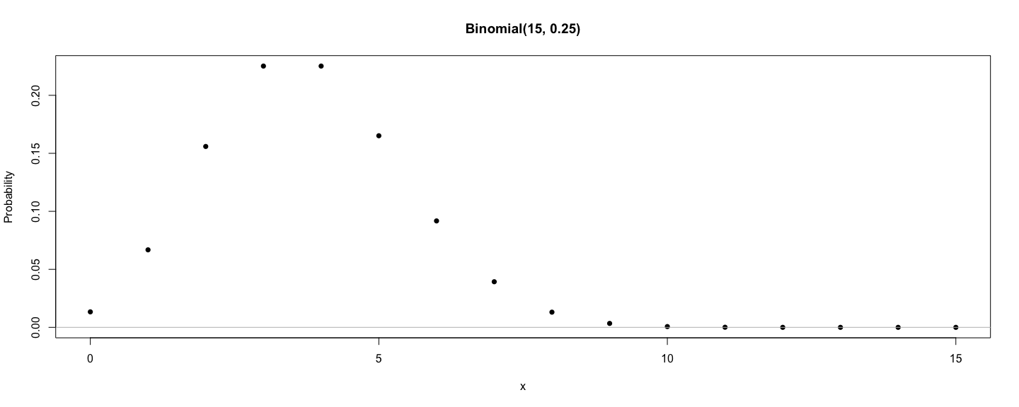
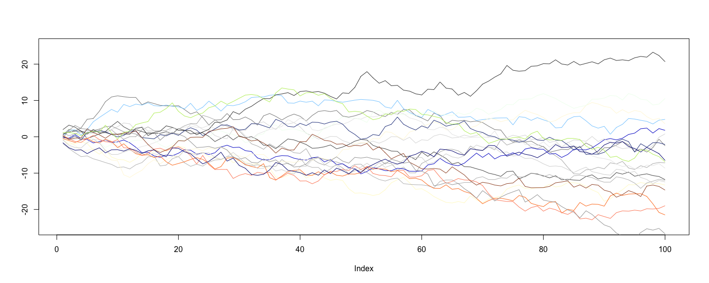
class: center, middle

# An Overview of R - 1

## Introductory Computer Programming

### Deepayan Sarkar

---

# Software for Statistics

- Computation is an essential part of modern statistics

- Handling large datasets

- Visualization

- Simulation

- Iterative methods

- Many softwares are available for such computation, but we will focus on R
--

- Why R?

- Available as [Free](https://en.wikipedia.org/wiki/Free_software_movement) / 
    	  [Open Source](https://en.wikipedia.org/wiki/The_Open_Source_Definition) Software

- Very popular (both academia and industry)

- Easy to try out on your own
--

- Also because I know R better than other languages

- Python and Julia are other good alternatives

---

# Outline

- Installing R (hopefully most of you have already done this)

- Basics of using R

- Some examples

---

# Installing R

* R is most commonly used as a [REPL](https://en.wikipedia.org/wiki/Read-eval-print_loop) (Read-Eval-Print-Loop)

* When it is started, R Waits for user input

* Evaluates and prints result

* Waits for more input
--

* There are several different _interfaces_ to do this

* R itself works on many platforms (Windows, Mac, UNIX, Linux)

* Some interfaces are platform-specific, some work on most
--

* R and the interface may need to be installed separately

---

# Installing R

* Go to <https://cran.r-project.org/> (or choose a [mirror](https://cran.r-project.org/mirrors.html) first)

* Follow instructions depending on your platform (Windows for most of you)
--

* This will install R, as well as a default graphical interface on Windows and Mac
--

* I will recommend a different interface called
  [R Studio](https://www.rstudio.com/) that needs to be installed separately
  
* I personally use yet another interface called
  [ESS](https://ess.r-project.org/) with a general-purpose
  editor called [Emacs](https://www.gnu.org/software/emacs/)

---

# Running R

* Once installed, you can start the appropriate interface (or R directly) to get something like this:

```
R version 4.0.3 (2020-10-10) -- "Bunny-Wunnies Freak Out"
Copyright (C) 2020 The R Foundation for Statistical Computing
Platform: x86_64-apple-darwin19.6.0 (64-bit)

R is free software and comes with ABSOLUTELY NO WARRANTY.
You are welcome to redistribute it under certain conditions.
Type 'license()' or 'licence()' for distribution details.

R is a collaborative project with many contributors.
Type 'contributors()' for more information and
'citation()' on how to cite R or R packages in publications.

Type 'demo()' for some demos, 'help()' for on-line help, or
'help.start()' for an HTML browser interface to help.
Type 'q()' to quit R.

> 
```

* The `>` represents a _prompt_ indicating that R is waiting for input.

* The difficult part is to learn what to do next

---

# The R REPL essentially works like a calculator

```r
34 * 23
```

```
[1] 782
```

```r
27 / 7
```

```
[1] 3.857143
```

```r
exp(2)
```

```
[1] 7.389056
```

```r
2^10
```

```
[1] 1024
```

---

# R has standard mathematical functions

```r
sqrt(5 * 125)
```

```
[1] 25
```

```r
log(120)
```

```
[1] 4.787492
```

```r
factorial(10)
```

```
[1] 3628800
```

```r
log(factorial(10))
```

```
[1] 15.10441
```

---

# R has standard mathematical functions

```r
choose(15, 5)
```

```
[1] 3003
```

```r
factorial(15) / (factorial(10) * factorial(5))
```

```
[1] 3003
```
--

```r
choose(1500, 2)
```

```
[1] 1124250
```

```r
factorial(1500) / (factorial(1498) * factorial(2))
```

```
[1] NaN
```

---

# R supports variables

```r
x <- 2
y <- 10
x^y
```

```
[1] 1024
```

```r
y^x
```

```
[1] 100
```

```r
factorial(y)
```

```
[1] 3628800
```

```r
log(factorial(y), base = x)
```

```
[1] 21.79106
```

---

# R can compute on vectors

```r
N <- 15
x <- seq(0, N)
N
```

```
[1] 15
```

```r
x
```

```
 [1]  0  1  2  3  4  5  6  7  8  9 10 11 12 13 14 15
```

```r
choose(N, x)
```

```
 [1]    1   15  105  455 1365 3003 5005 6435 6435 5005 3003 1365  455  105   15    1
```

---

# R has functions for statistical calculations

```r
p <- 0.25
choose(N, x) * p^x * (1-p)^(N-x)
```

```
 [1] 1.336346e-02 6.681731e-02 1.559070e-01 2.251991e-01 2.251991e-01 1.651460e-01 9.174777e-02
 [8] 3.932047e-02 1.310682e-02 3.398065e-03 6.796131e-04 1.029717e-04 1.144130e-05 8.800998e-07
[15] 4.190952e-08 9.313226e-10
```

```r
dbinom(x, size = N, prob = p)
```

---

# R has functions that work on vectors

```r
p.x <- dbinom(x, size = N, prob = p)
sum(x * p.x) / sum(p.x)
```

```
[1] 3.75
```

```r
N * p
```

```
[1] 3.75
```

---

# R can draw graphs

```r
plot(x, p.x, ylab = "Probability", pch = 16)
title(main = sprintf("Binomial(%g, %g)", N, p))
abline(h = 0, col = "grey")
```

![plot of chunk unnamed-chunk-9](figures/roverview-1-unnamed-chunk-9-1.png)
\

---

# R can simulate random variables

```r
cards <- as.vector(outer(c("H", "D", "C", "S"), 1:13, paste))
cards
```

```
 [1] "H 1"  "D 1"  "C 1"  "S 1"  "H 2"  "D 2"  "C 2"  "S 2"  "H 3"  "D 3"  "C 3"  "S 3"  "H 4" 
[14] "D 4"  "C 4"  "S 4"  "H 5"  "D 5"  "C 5"  "S 5"  "H 6"  "D 6"  "C 6"  "S 6"  "H 7"  "D 7" 
[27] "C 7"  "S 7"  "H 8"  "D 8"  "C 8"  "S 8"  "H 9"  "D 9"  "C 9"  "S 9"  "H 10" "D 10" "C 10"
[40] "S 10" "H 11" "D 11" "C 11" "S 11" "H 12" "D 12" "C 12" "S 12" "H 13" "D 13" "C 13" "S 13"
```
--

```r
sample(cards, 13)
```

```
 [1] "D 4"  "D 1"  "D 7"  "D 9"  "C 8"  "H 12" "S 12" "D 8"  "S 9"  "H 2"  "D 6"  "C 4"  "H 5" 
```

```r
sample(cards, 13)
```

```
 [1] "C 5"  "S 6"  "S 9"  "S 3"  "C 12" "D 9"  "D 3"  "C 8"  "D 4"  "S 8"  "C 7"  "D 2"  "S 11"
```

---

# R can simulate random variables

```r
z <- rnorm(50, mean = 0, sd = 1)
z
```

```
 [1] -0.35881905 -1.03417675 -1.33638696 -1.66146785 -0.96042670  0.67585936  0.57335724 -1.87385190
 [9] -0.40798688  0.57243941  0.16057616  0.02660315  0.64993229  1.15937452 -0.17677525  0.82469443
[17] -0.29641834 -0.91972462 -1.77191374  0.75219387 -1.42906152 -0.52755159  1.72622568 -0.05394051
[25] -1.99618976  1.66291284  0.42827317  1.37329212  0.35032933  1.02496673 -1.54762037 -0.10031568
[33] -0.78021340 -0.83779551  0.25937539  0.25027196 -0.93206311 -1.16235345 -0.08591635  0.87588717
[41] -0.31723365 -0.45890017 -1.01457091  0.90673169  0.46920924  1.78821720 -0.49774941  0.49501141
[49] -2.81175862 -0.48808573
```

---

# Example: random walk

```r
plot(1:100, type = "n", ylim = c(-25, 25), ylab = "")
for (i in 1:20) {
    z <- rnorm(100, mean = 0, sd = 1)
    lines(cumsum(z), col = sample(colors(), 1))
}
```

![plot of chunk unnamed-chunk-13](figures/roverview-1-unnamed-chunk-13-1.png)
\

---

# R is in fact a full programming language

* Variables

* Functions

* Control flow structures

* For loops, while loops

* If-then-else (branching)
--

* Distinguishing features

* Focus on _vectors_ and _vectorized operations_

* Treatment of _functions_ at par with other object types

* We will next see a few examples to illustrate what I mean by this