COVID-19 in the US states

Deepayan Sarkar

TARGET.cases <- "time_series_covid19_confirmed_US.csv"
TARGET.deaths <- "time_series_covid19_deaths_US.csv"
SURL <- "https://github.com/CSSEGISandData/COVID-19/raw/master/csse_covid_19_data/csse_covid_19_time_series"
## To download the latest version, delete the files and run again
for (target in c(TARGET.cases, TARGET.deaths))
{
	if (!file.exists(target))
        download.file(sprintf("%s/%s", SURL, target), destfile = target)
}

[This note was last updated using data downloaded on 2020-08-25. Here is the source of this analysis. Click here to show / hide the R code used. ]

covid.cases <- read.csv(TARGET.cases, check.names = FALSE, stringsAsFactors = FALSE)
covid.deaths <- read.csv(TARGET.deaths, check.names = FALSE, stringsAsFactors = FALSE)
## covid.deaths has an extra column called Population, which we drop for now
covid.deaths$Population <- NULL
if (!identical(colnames(covid.deaths), colnames(covid.cases)))
{
    warning("Cases and death data have different columns (dates)... using common ones.")
    common.colnames <- intersect(colnames(covid.deaths), colnames(covid.cases))
    covid.deaths <- covid.deaths[colnames(covid.deaths) %in% common.colnames]
    covid.cases <- covid.cases[colnames(covid.cases) %in% common.colnames]
}
if (!identical(rownames(covid.cases), rownames(covid.deaths)))
{
    stop("Cases and death data have different rows... check versions.")
}
omit.regions <- c("Diamond Princess", "Grand Princess")
covid.deaths <- subset(covid.deaths, !(Province_State %in% omit.regions))
covid.cases <- subset(covid.cases, !(Province_State %in% omit.regions))

correctLag <- function(x)
{
    n <- length(x)
    stopifnot(n > 2)
    for (i in seq(2, n-1))
        if (x[i] == x[i-1])
            x[i] <- sqrt(x[i-1] * x[i+1])
    x
}
extractCasesTS <- function(d)
{
    x <- t(data.matrix(d[, -c(1:11)]))
    x[x == -1] <- NA
    colnames(x) <- with(d, paste(Province_State, Admin2, sep = " / "))
    apply(x, 2, correctLag)
}
tdouble <- function(x)
{
    if (all(x == 0)) return (NA)
    x <- c(0, x[x > 0])
    i <- seq_along(x)
    f <- approxfun(x, i)
    diff(f(max(x) * c(0.5, 1)))
}

By state

## State-wise totals
byState.cases <- split(covid.cases, covid.cases$Province_State)
byState.deaths <- split(covid.deaths, covid.deaths$Province_State)
state.cases <- sapply(byState.cases, function(d) colSums(data.matrix(d[, -c(1:11)])))
state.deaths <- sapply(byState.deaths, function(d) colSums(data.matrix(d[, -c(1:11)])))
D <- nrow(state.cases)

The following plot shows the current doubling time for deaths and cases, across US states, with states sorted by the total number of deaths.

stotal.deaths <- state.deaths[D, , drop = TRUE]
stotal.cases <- state.cases[D, , drop = TRUE]
sdt.deaths <- apply(state.deaths, 2, tdouble)
sdt.cases <- apply(state.cases, 2, tdouble)
state.names <- names(sdt.deaths)
state.names <- factor(state.names, levels = state.names,
                      labels = sprintf("%s (%g)", state.names, stotal.deaths))
dotplot(reorder(state.names, stotal.deaths) ~ sdt.deaths + sdt.cases,
        scales = list(alternating = 3), xlab = "Doubling time in days",
        par.settings = simpleTheme(pch = 16),
        auto.key = list(space = "right", text = c("Deaths", "Cases")))

plot of chunk unnamed-chunk-5

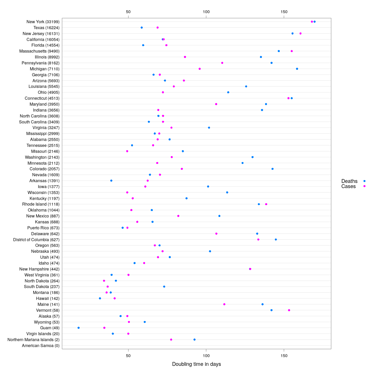
Generally speaking, the doubling times for cases are higher than that for days. This is a good indicator: as deaths lag behind cases, we can expect that around a week from now, the doubling time for deaths will increase to make up the difference.

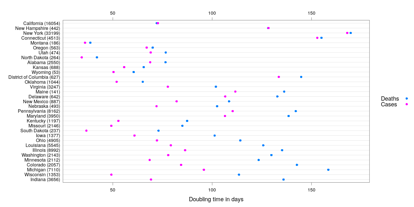
The following states are somewhat poor performers in this respect: they have more than 40 deaths, and the difference in their doubling times is less that 2 days (although Washington is doing pretty well in terms of the absolute doubling times).

dotplot(reorder(state.names, sdt.cases - sdt.deaths) ~ sdt.deaths + sdt.cases,
        subset = (sdt.cases - sdt.deaths < 2 & stotal.deaths > 40),
        scales = list(alternating = 3), xlab = "Doubling time in days",
        par.settings = simpleTheme(pch = 16),
        auto.key = list(space = "right", text = c("Deaths", "Cases")))

plot of chunk unnamed-chunk-6

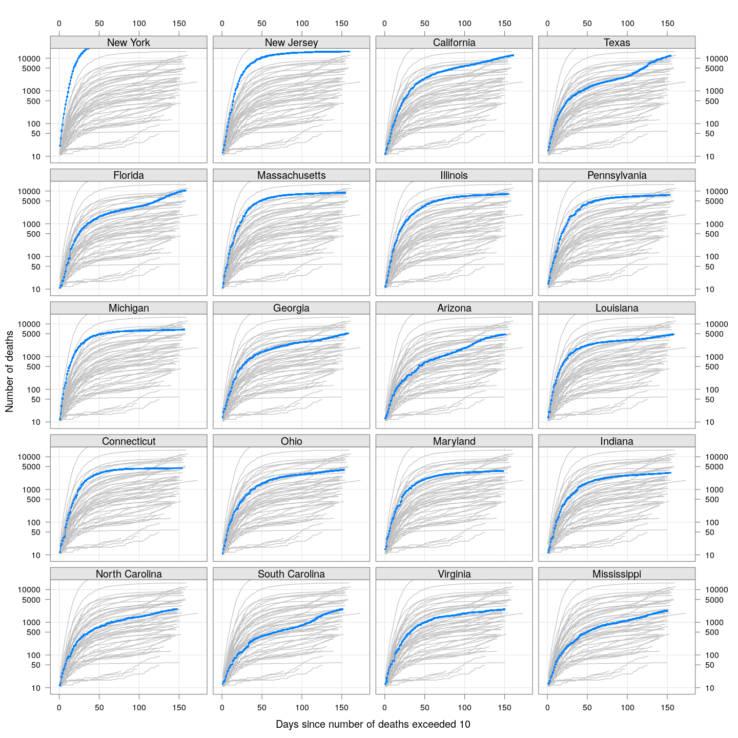
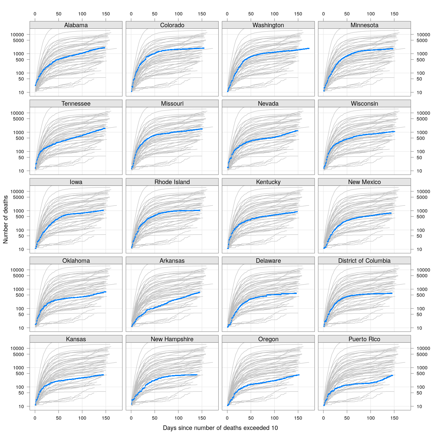
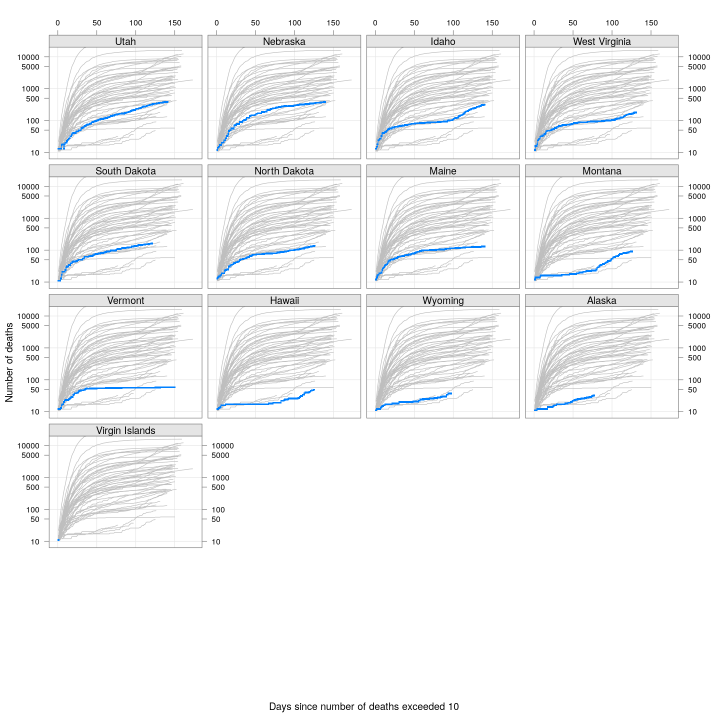
The following plots show how the number of deaths have grown in these states since the count first exceeded 50, compared to the other counties.

deathsSince10 <- function(region, xdata)
{
    x <- xdata[, region, drop = TRUE]
    x <- x[x > 10]
    if (length(x) == 0) return (NULL)
    data.frame(region = region, day = seq_along(x),
               deaths = x, total = tail(x, 1))
}
panel.glabel <- function(x, y, group.value, col.symbol, ...) # x,y vectors; group.value scalar
{
    n <- length(x)
    panel.text(x[n], y[n], label = group.value, pos = 4, col = col.symbol, srt = 40)
}
deaths.10 <- do.call(rbind, lapply(colnames(state.deaths), deathsSince10,
                                   xdata = state.deaths))
bg <- xyplot(deaths ~ day, data = deaths.10, grid = TRUE,
             scales = list(alternating = 3, y = list(log = 10, equispaced.log = FALSE)),
             col = "grey", groups = region, type = "l")
fg <- 
    xyplot(deaths ~ day | reorder(region, -total), data = deaths.10,
           xlab = "Days since number of deaths exceeded 10",
           ylab = "Number of deaths", pch = ".", cex = 3, 
           scales = list(alternating = 3, y = list(log = 10, equispaced.log = FALSE)),
           as.table = TRUE, between = list(x = 0.5, y = 0.5), layout = c(4, 5),
           type = "o", ylim = c(NA, 20000))
fg + as.layer(bg, under = TRUE)

plot of chunk unnamed-chunk-7

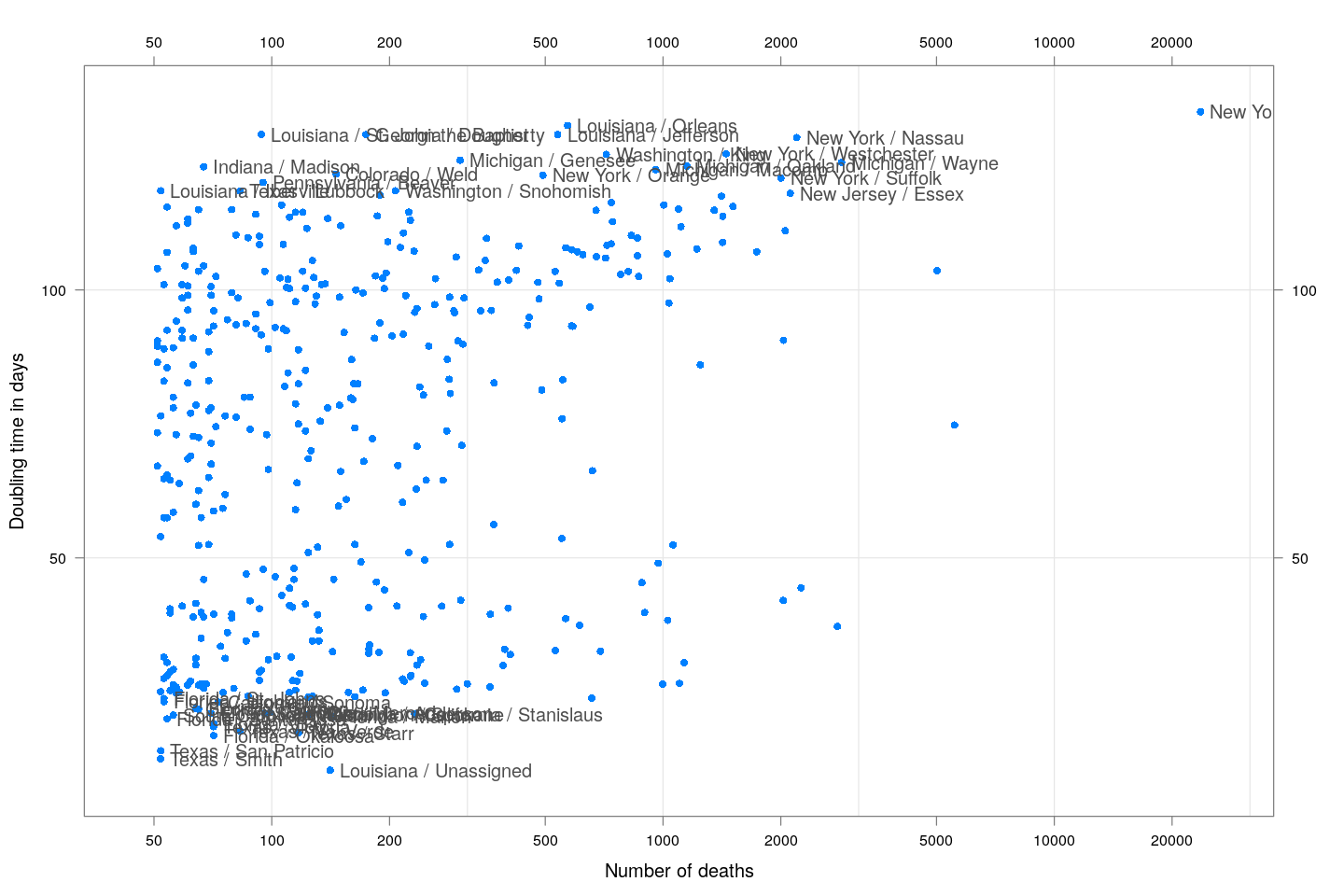
By county or other administrative region

Most cases are concentrated in some specific counties. The following plot gives the current doubling time of deaths, compared to total number of deaths, across US counties / regions with at least 50 deaths.

keep <- covid.deaths[[length(covid.deaths)]] > 50 # at least 50 deaths
covid.cases <- covid.cases[keep, ]
covid.deaths <- covid.deaths[keep, ]
xcovid.cases <- extractCasesTS(covid.cases)
xcovid.deaths <- extractCasesTS(covid.deaths)
D <- nrow(xcovid.deaths)
total.deaths <- xcovid.deaths[D, , drop = TRUE]
dt.deaths <- apply(xcovid.deaths, 2, tdouble)
do.label.1 <- dt.deaths < quantile(dt.deaths, 0.05, na.rm = TRUE) | dt.deaths > quantile(dt.deaths, 0.95, na.rm = TRUE)
do.label.2 <- (total.deaths > max(total.deaths)/2) & !(do.label.1)
xyplot(dt.deaths ~ total.deaths, pch = 16, grid = TRUE,
       ylab = "Doubling time in days", xlab = "Number of deaths",
       scales = list(alternating = 3, x = list(log = 10, equispaced.log = FALSE))) +
    layer(panel.text(x[do.label.1], y[do.label.1],
                     labels = names(total.deaths)[do.label.1],
                     pos = 4, col = "grey30")) + 
    layer(panel.text(x[do.label.2], y[do.label.2],
                     labels = names(total.deaths)[do.label.2],
                     pos = 2, col = "grey30"))

plot of chunk unnamed-chunk-8

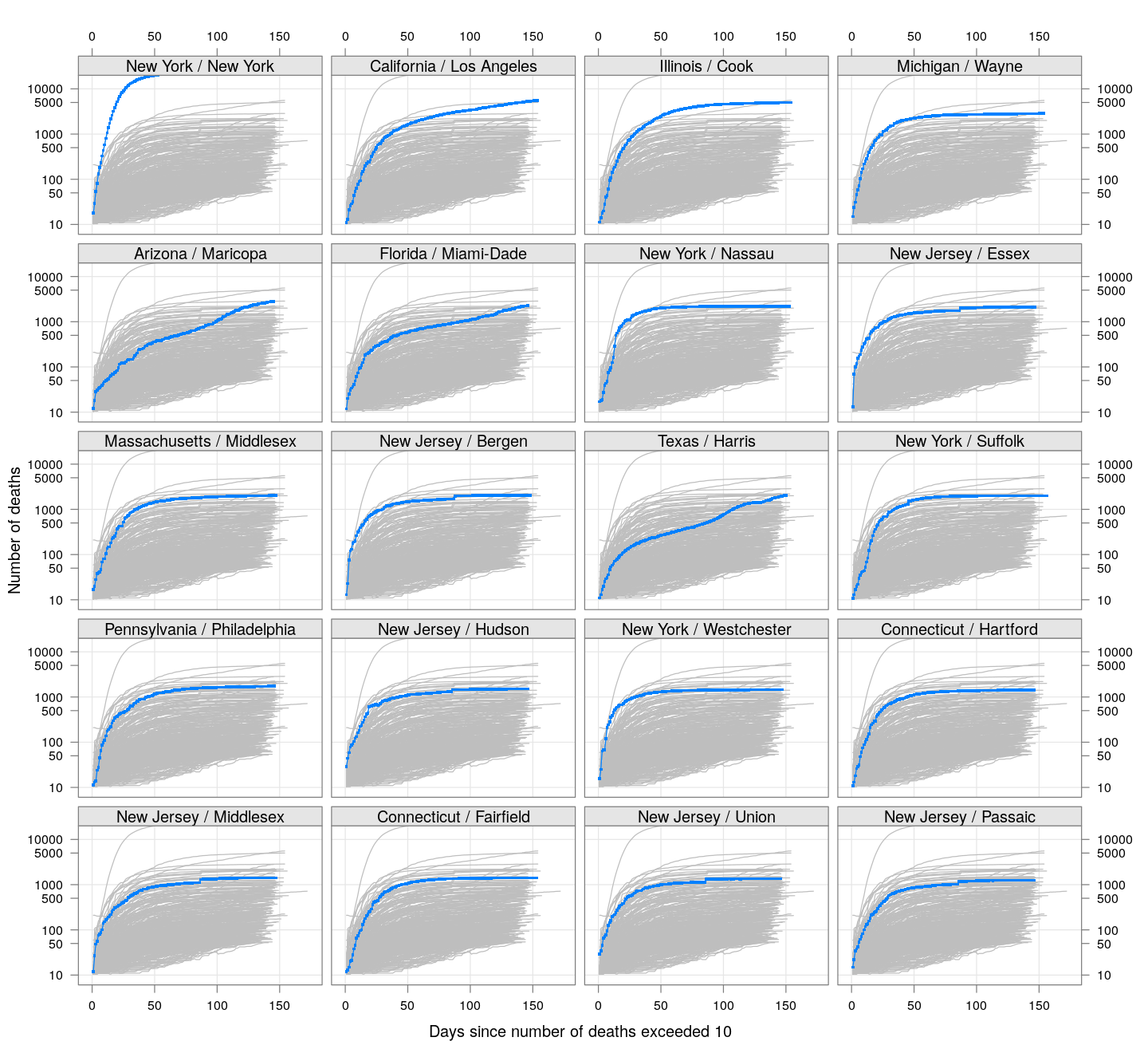
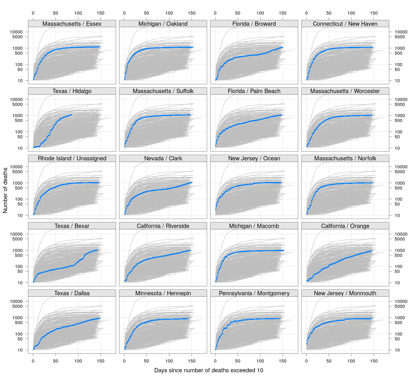
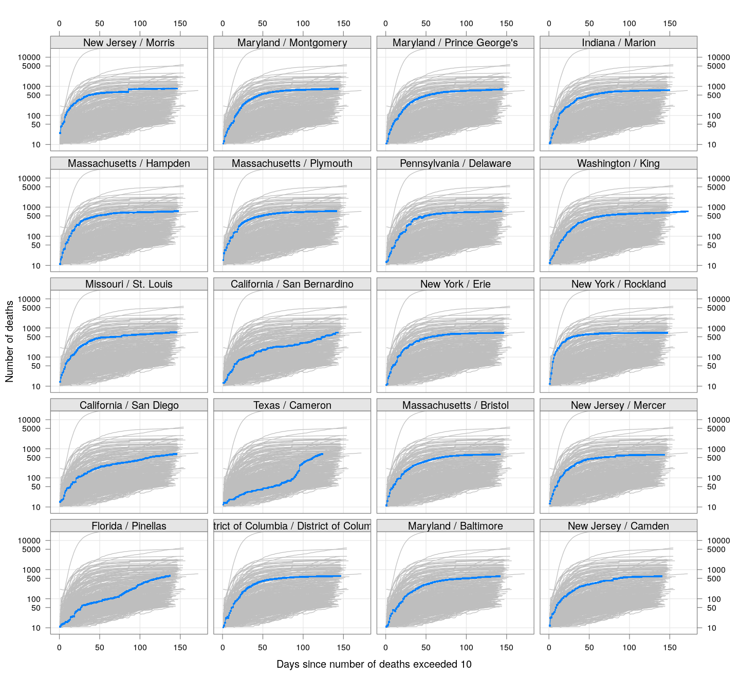
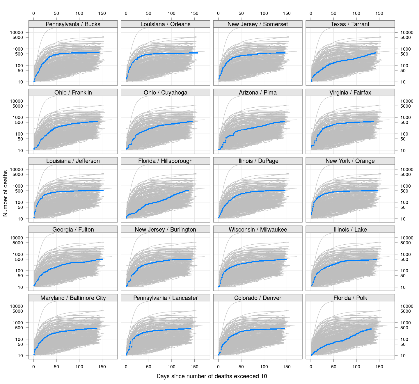
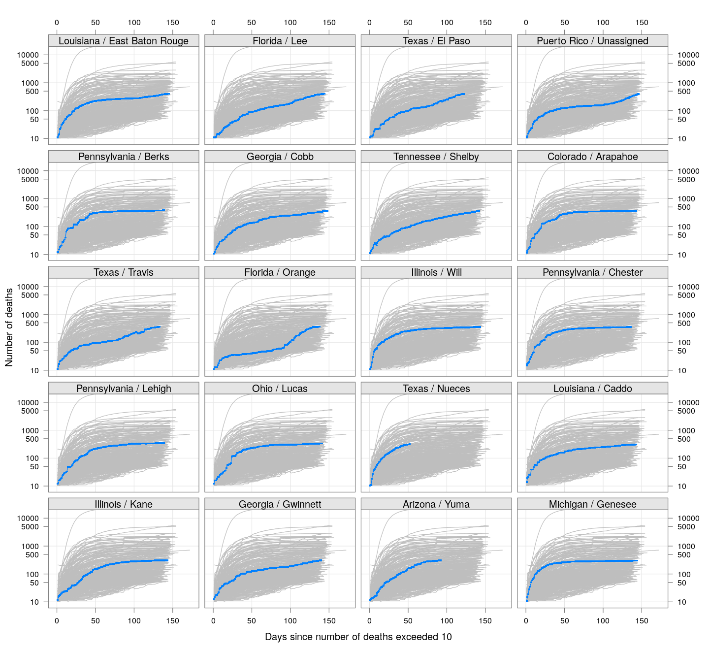
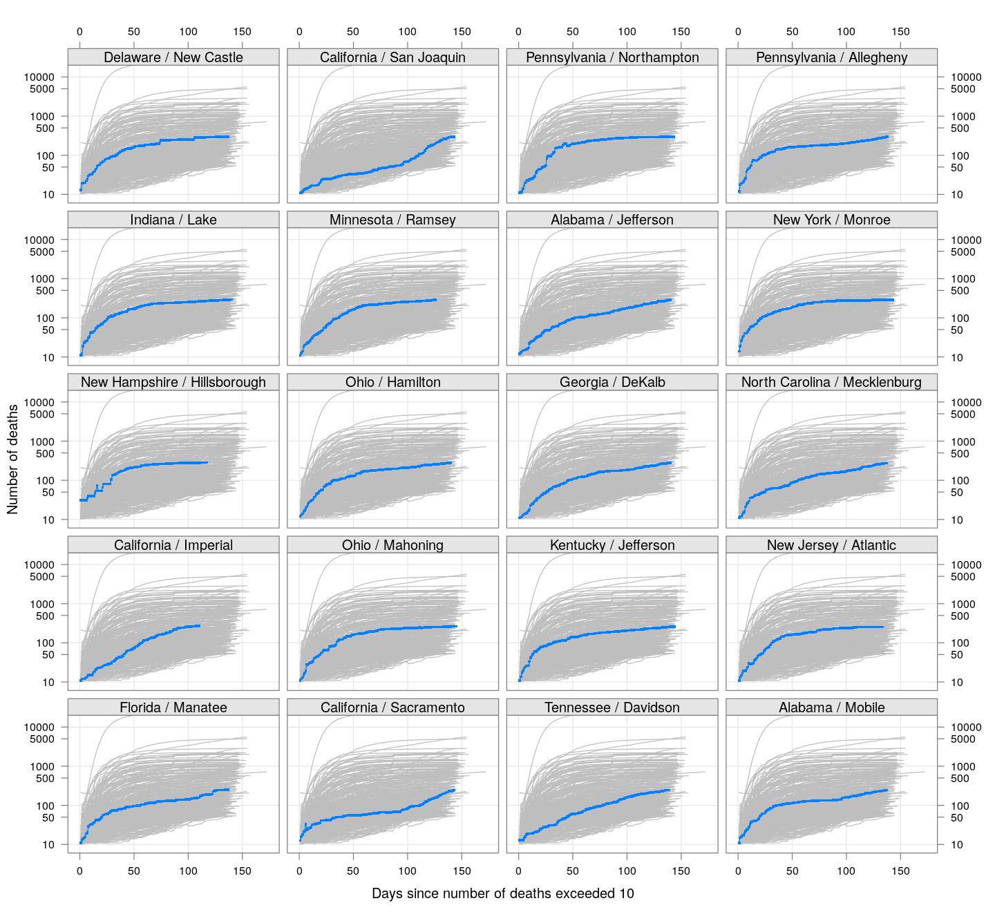
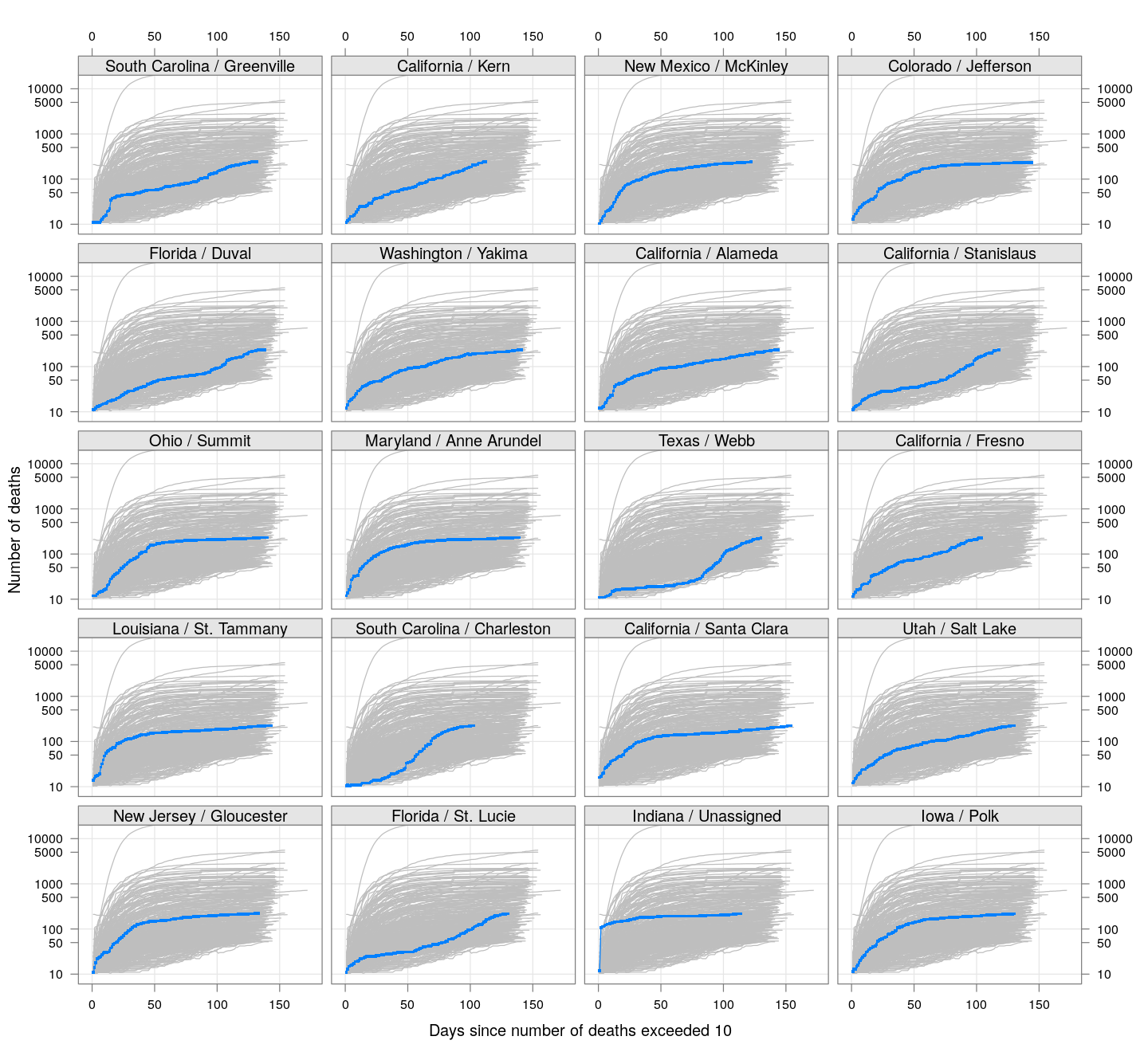
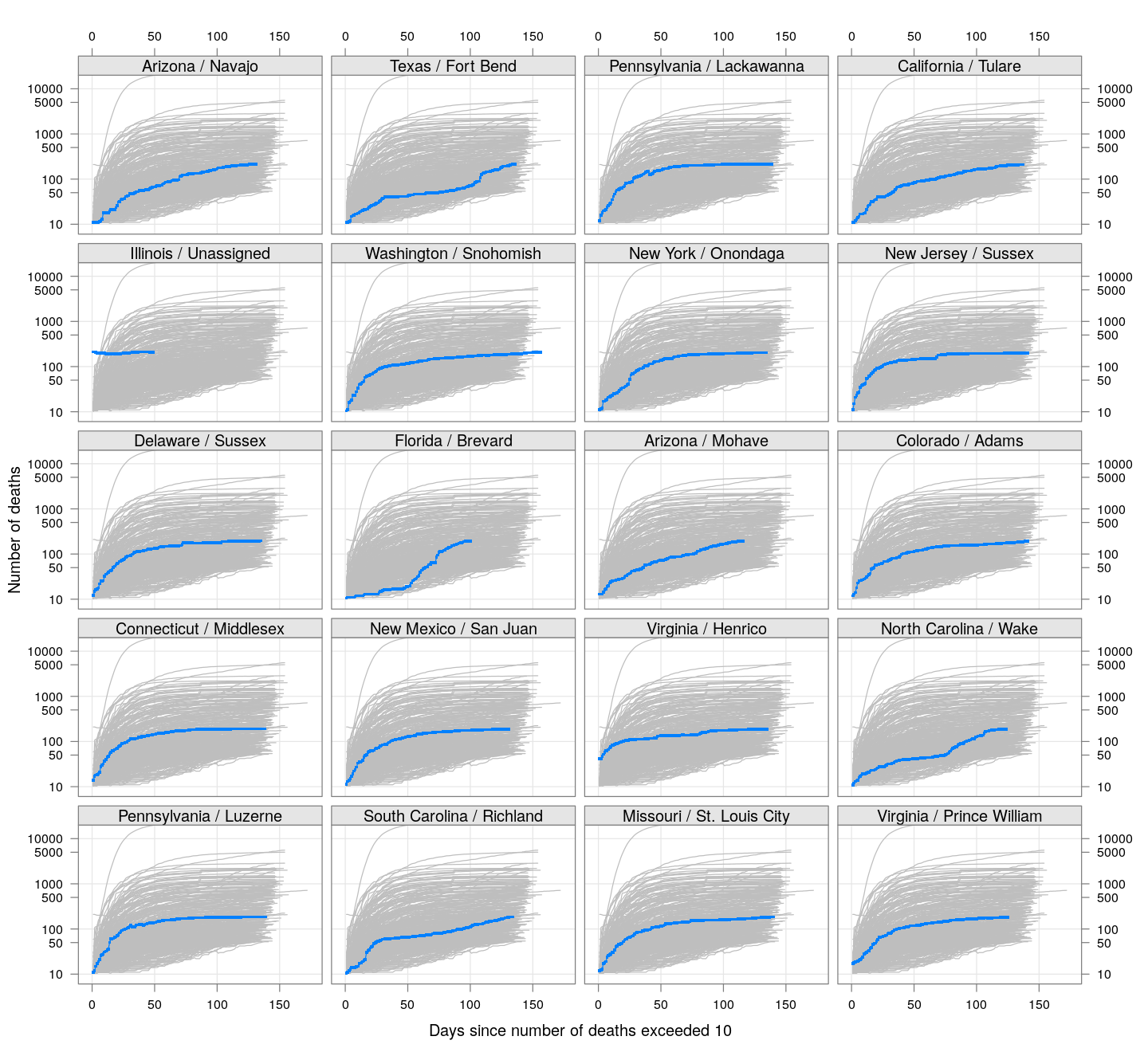
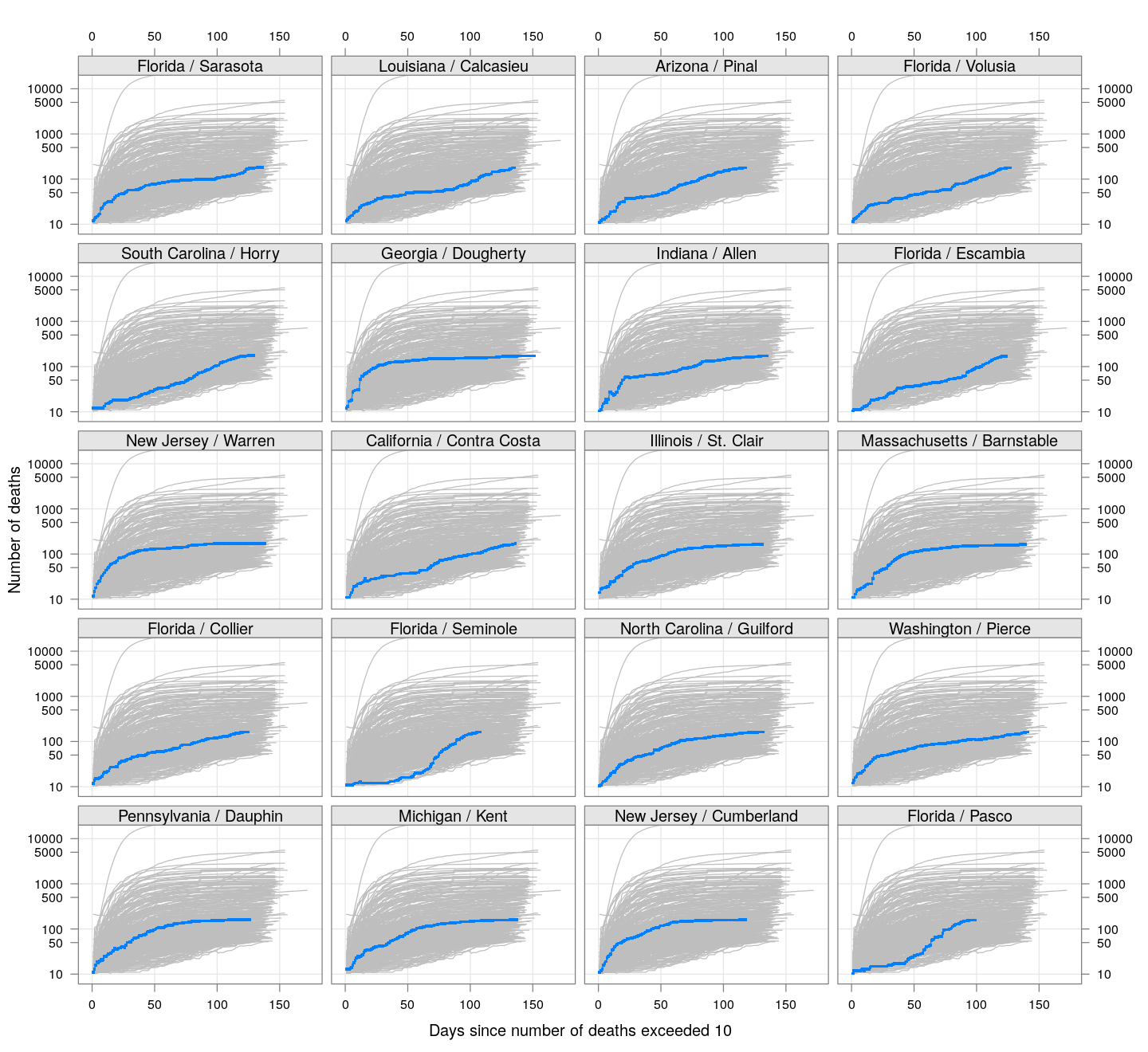
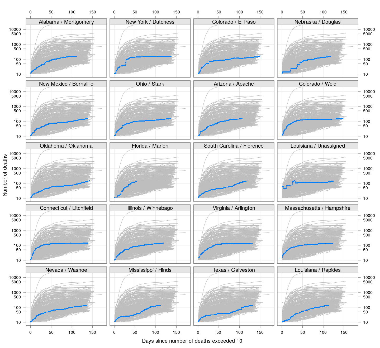
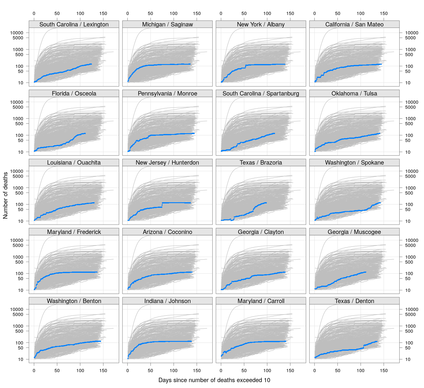
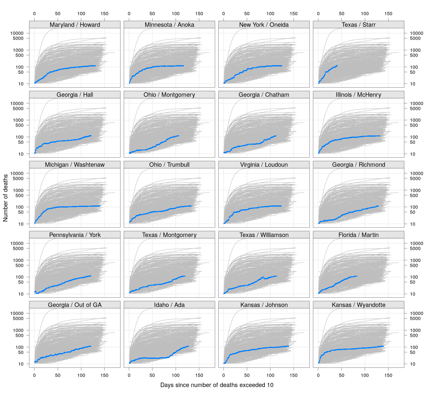
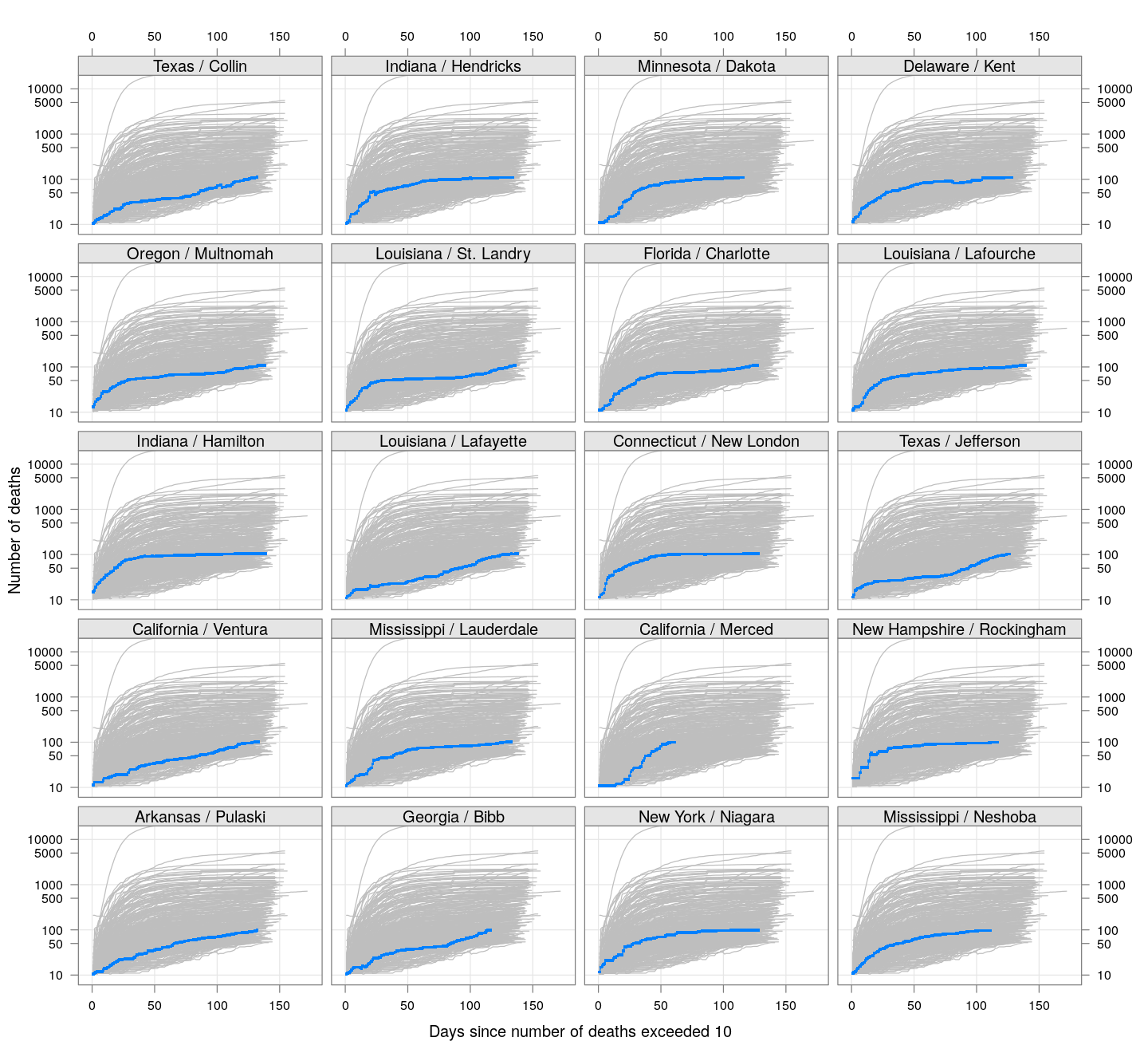
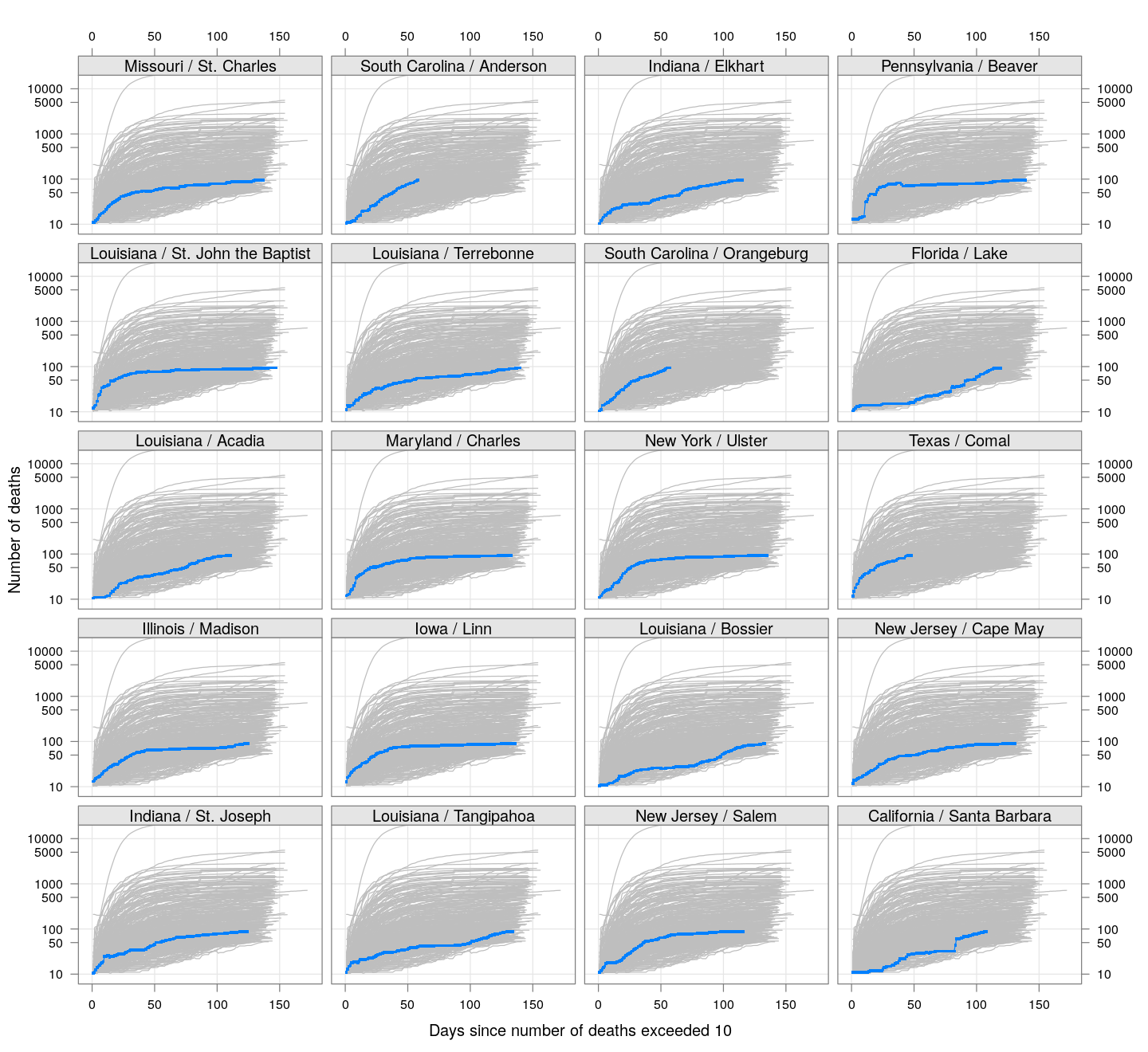
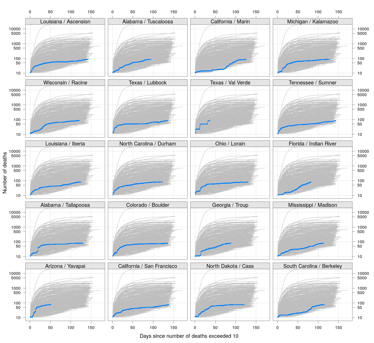
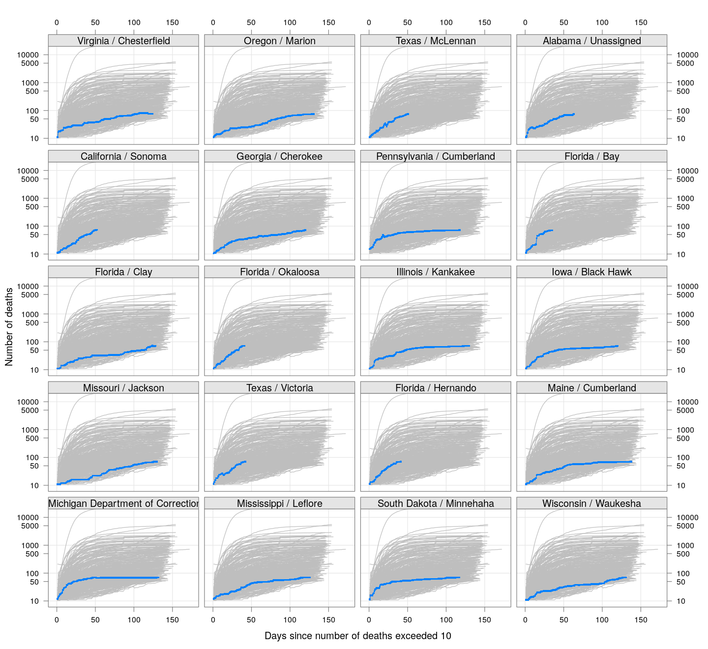
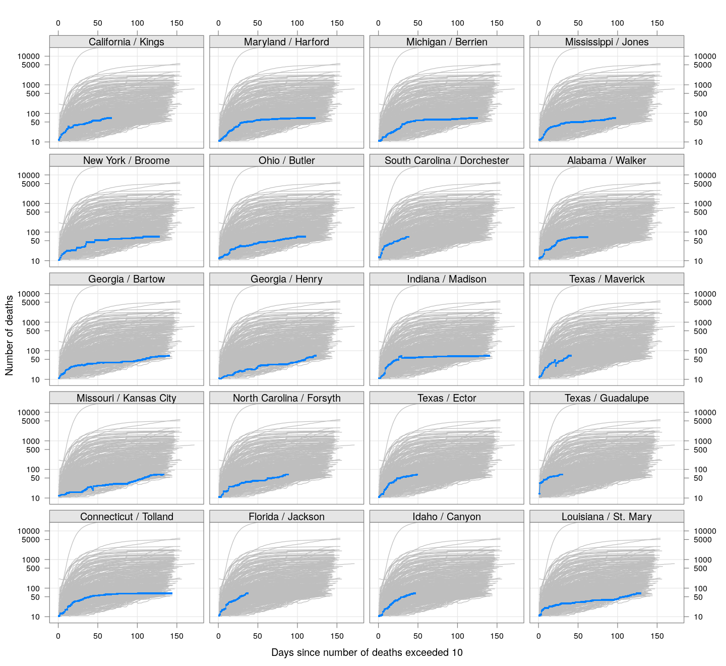
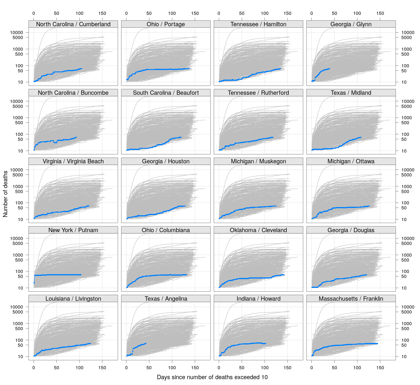
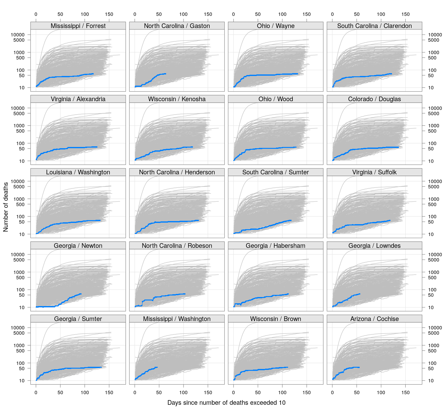
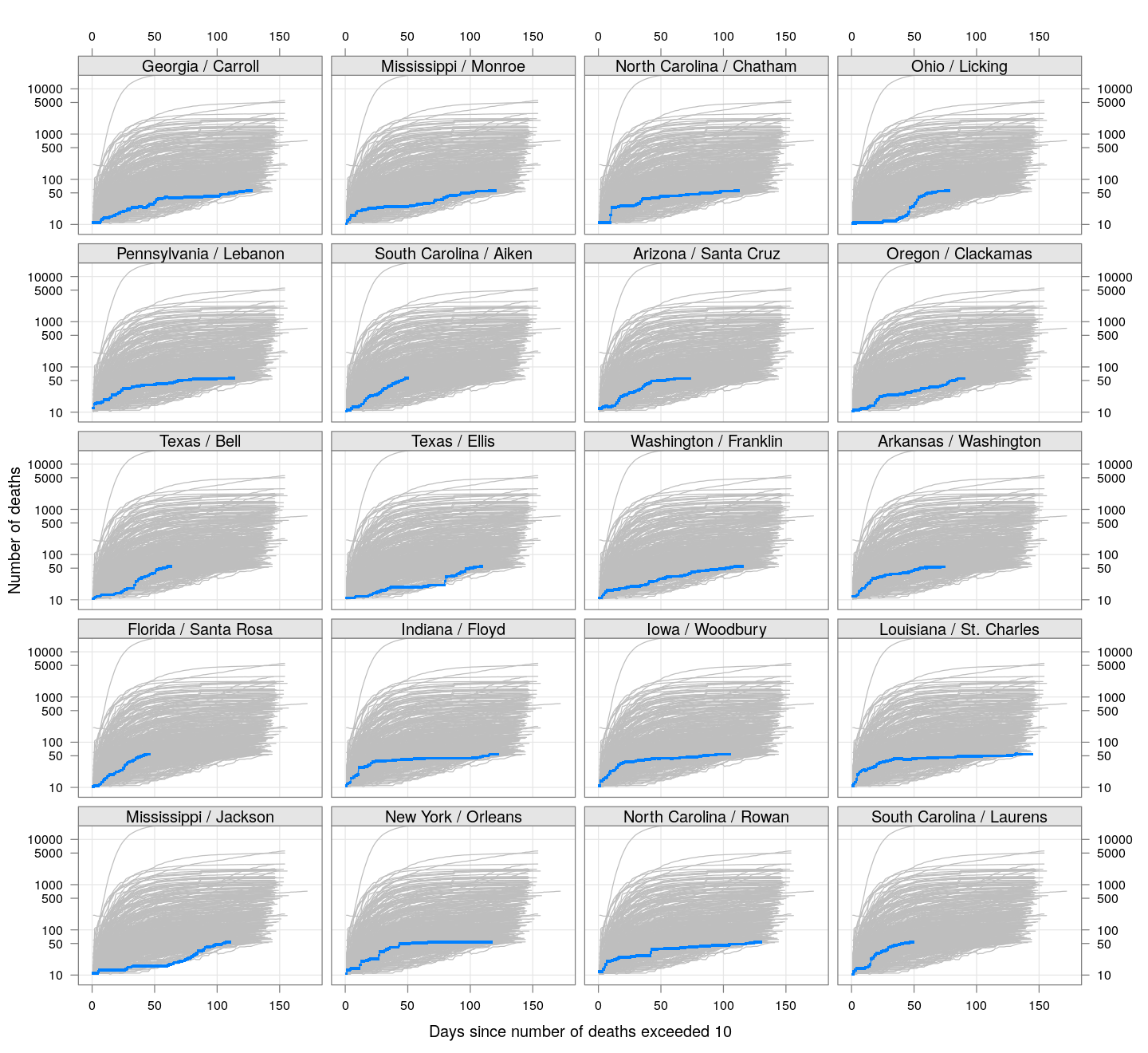
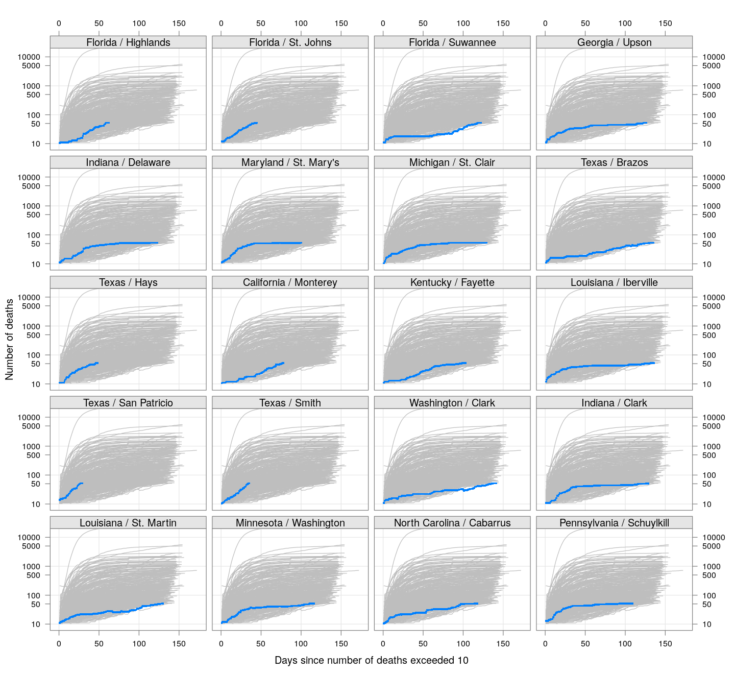
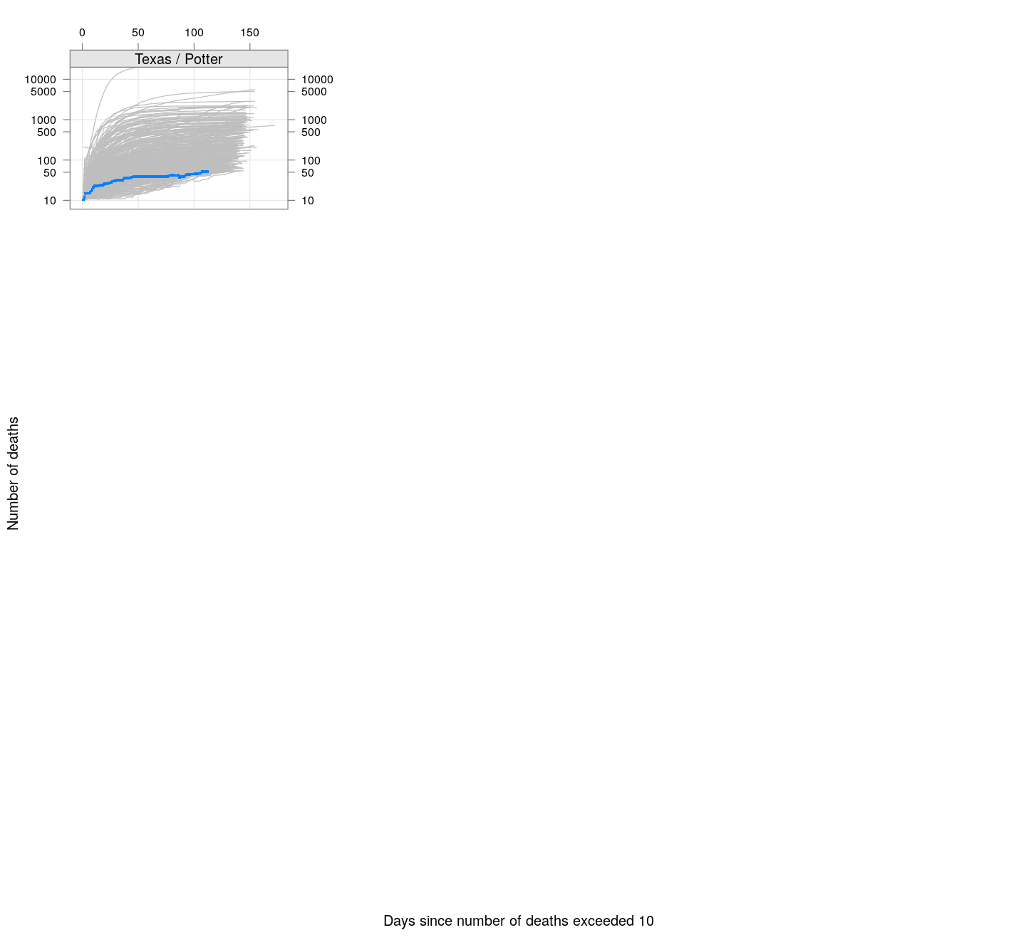
The following plots show how the number of deaths have grown in these counties since the count first exceeded 50, compared to the other counties.

deaths.10 <- do.call(rbind, lapply(colnames(xcovid.deaths), deathsSince10,
                                   xdata = xcovid.deaths))
bg <- xyplot(deaths ~ day, data = deaths.10, grid = TRUE,
             scales = list(alternating = 3, y = list(log = 10, equispaced.log = FALSE)),
             col = "grey", groups = region, type = "l")
fg <- 
    xyplot(deaths ~ day | reorder(region, -total), data = deaths.10,
           xlab = "Days since number of deaths exceeded 10",
           ylab = "Number of deaths", pch = ".", cex = 3, 
           scales = list(alternating = 3, y = list(log = 10, equispaced.log = FALSE)),
           as.table = TRUE, between = list(x = 0.5, y = 0.5), layout = c(4, 5),
           type = "o", ylim = c(NA, 20000))
fg + as.layer(bg, under = TRUE)

plot of chunk unnamed-chunk-9