REPL

• R works using what is known as a REPL (Read-Eval-Print-Loop)

  • R waits for user input when it starts

  • User types input expression and presses Enter

  • R reads input and tries to evaluate

  • Evaluation is either successful or produces an error

  • R starts to wait again for further user input

• Today's talk takes a closer look at how the evaluation step works

REPL

• R works using what is known as a REPL (Read-Eval-Print-Loop)

  • R waits for user input when it starts

  • User types input expression and presses Enter

  • R reads input and tries to evaluate

  • Evaluation is either successful or produces an error

  • R starts to wait again for further user input

• Today's talk takes a closer look at how the evaluation step works

• Useful links: Source (R + Markdown), Makefile (conversion using knitr and pandoc), Extracted R code

Prerequisites

• Basic R programming

  • You should be comfortable with writing functions

  • If you know how to use eval() and quote(), you already know too much

• Statistical concepts used for illustration

  • Maximum likelihood, regularization

  • Probability density, histograms

  • Linear regression

Evaluation

• Consider the following expression that we wish to evaluate

sqrt(x)

Error in eval(expr, envir, enclos): object 'x' not found

• This expression involves two "symbols", sqrt and x

• To be able to evaluate the expression, R must be able to "find" both symbols

find("sqrt")

[1] "package:base"

find("x") # not found

character(0)

Evaluation

• So let us define x and try again

x <- 10
sqrt(x)

[1] 3.162278

x <- -1
sqrt(x)

Warning in sqrt(x): NaNs produced

[1] NaN

Evaluation

x <- -1+0i
sqrt(x)

[1] 0+1i

x <- "-1"
sqrt(x)

Error in sqrt(x): non-numeric argument to mathematical function

Evaluation

• Let us check again where sqrt and x are found

find("sqrt")

[1] "package:base"

find("x")

[1] ".GlobalEnv"

Evaluation

• Suppose we want to define a "smarter" sqrt()

• First check what sqrt() does, so we can mimic:

sqrt

function (x)  .Primitive("sqrt")

• What does .Primitive() do? See help(.Primitive) (but we don't really need to know)

Evaluation

• Define a "smart" sqrt() as follows:

sqrt <- function(x)
{
    orig.sqrt <- .Primitive("sqrt")
    if (is.character(x)) x <- as.numeric(x)
    if (is.numeric(x) && any(x < 0)) x <- complex(real = x, imaginary = 0)
    orig.sqrt(x)
}

• We now have

x <- -1
sqrt(x)

[1] 0+1i

Multiple symbol definitions

• Where is R finding these symbols?

find("x")

[1] ".GlobalEnv"

find("sqrt")

[1] ".GlobalEnv"   "package:base"

• Note that the "original" sqrt() is not overwritten; instead a new one is defined

The search path

• Why is it using the sqrt in ".GlobalEnv" and not the one in "package:base"?

search()

 [1] ".GlobalEnv"        "package:knitr"     "package:stats"     "package:graphics" 
 [5] "package:grDevices" "package:utils"     "package:datasets"  "package:methods"  
 [9] "Autoloads"         "package:base"

• R searches for symbols sequentially in the "search path"

Environments

• What exactly are the objects in the search path?

• They are known as "environments", which are central to how evaluation works in R

• In essence, an environment is a collection of symbols (variables) bound to certain values

• Each environment usually also has an associated "enclosing environment" or "parent environment"

• .GlobalEnv is the environment where user-defined variables are stored

Environments

• The chain of enclosing environments starting from .GlobalEnv is identical to the search path

e <- .GlobalEnv
while (TRUE) { str(e, give.attr = FALSE); e <- parent.env(e) }

<environment: R_GlobalEnv> 
<environment: package:knitr> 
<environment: package:stats> 
<environment: package:graphics> 
<environment: package:grDevices> 
<environment: package:utils> 
<environment: package:datasets> 
<environment: package:methods> 
<environment: 0x7f9063aa8bb8> 
<environment: base> 
<environment: R_EmptyEnv>

Error in parent.env(e): the empty environment has no parent

search() # compare

 [1] ".GlobalEnv"        "package:knitr"     "package:stats"     "package:graphics" 
 [5] "package:grDevices" "package:utils"     "package:datasets"  "package:methods"  
 [9] "Autoloads"         "package:base"

Creating and manipulating environments

• new.env() explicitly creates environments

• Variables inside environments can be accessed using $ (like lists or data frames)

e1 <- new.env()
e1$x <- seq(0, 2 * pi, length.out = 101)
e1$y <- cos(e1$x)
plot(y ~ x, data = e1, type = "l", ylim = c(-1, 1)) # Formula interface

Environments are not duplicated when copied

• Environments are an exception to R's duplicate-on-copy rule

• A copy of an environment is the same environment, not a new one

e2 <- e1
range(e1$y)

[1] -1  1

e2$y <- abs(e2$y)
range(e1$y) # changes even though e1$y has not been directly modified

[1] 1.608123e-16 1.000000e+00

Inspecting the variables in an environment

• The names of objects available in an environment can be obtained by ls()

ls(e2)

[1] "x" "y"

ls.str(e2) ## summary of all objects in e2

x :  num [1:101] 0 0.0628 0.1257 0.1885 0.2513 ...
y :  num [1:101] 1 0.998 0.992 0.982 0.969 ...

Environments and functions

• Environments are central to how R functions work

• Functions in R are actually "closures"

• In addition to the argument list and body (code), a function also has an associated environment

• This is usually the environment in which the function was defined

environment(sqrt)

<environment: R_GlobalEnv>

environment(base::sqrt) # special "primitive" (C) function, so no environment

NULL

environment(hist)

<environment: namespace:graphics>

What happens when a function is executed?

• Every time a function is invoked, a new environment is created

• This is the "evaluation environment" and contains the local variables of the function

• The environment of the function is the environment enclosing this "evaluation environment"

What happens when a function is executed?

• Every time a function is invoked, a new environment is created

• This is the "evaluation environment" and contains the local variables of the function

• The environment of the function is the environment enclosing this "evaluation environment"

• While the function is running, evaluation tries to find symbols as follows:

  • First, in the evaluation environment

  • Next, in its enclosing environment, i.e., the environment of the function

  • Then, in the enclosing environment of that environment, and so on

• This behaviour is called "lexical scoping"

What happens when a function is executed?

• Every time a function is invoked, a new environment is created

• This is the "evaluation environment" and contains the local variables of the function

• The environment of the function is the environment enclosing this "evaluation environment"

• While the function is running, evaluation tries to find symbols as follows:

  • First, in the evaluation environment

  • Next, in its enclosing environment, i.e., the environment of the function

  • Then, in the enclosing environment of that environment, and so on

• This behaviour is called "lexical scoping"

• Evaluation in the global environment follows the same rule (hence the search path)

Are these details important to know?

• Depends!

• You can use R productively with only a superficial understanding of evaluation

• However, these details often help explain and diagnose seemingly odd behaviour

• They can also be a lot of fun

Example: The Box-Cox transformation

• Given positive-valued (possibly skewed) data, one may want to transform them to look Normal

• The Box-Cox transformation conveniently combines power transforms and log in a single family

• Parameterized by a single parameter $\lambda$

Scoping rules can mask errors

• Consider the following function (which uses an undefined variable lambda)

boxcox <- function(x) # applies Box-Cox transformation on data 'x'
{
    if (lambda == 0) log(x)
    else (x^lambda - 1) / lambda
}
b <- function(x) # computes histogram bins given data 'x' 
{
    n <- sum(is.finite(x))
    r <- extendrange(x)
    seq(r[1], r[2], length.out = round(sqrt(n)) + 1)
}

x <- rlnorm(1000)
hist(boxcox(x), breaks = b) # error, as it should be

Error in boxcox(x): object 'lambda' not found

Scoping rules can mask errors

• The same code will "work" if lambda happens to be defined

lambda <- 0
hist(boxcox(x), breaks = b)  # notice that 'b' is a function! (See ?hist)

But sometimes we want to write such functions

• Normally, depending on this kind of scoping behaviour should be unnecessary

• In fact, a well-designed function should not depend on arbitrary variables

• However, there is one situation where this evaluation rule becomes important

• When a function creates and returns or uses another function!

Do we need functions that create functions?

• Probably not very common...

• But only because we are limited in our thinking

• We already use functions as arguments to other functions

• Thinking "functionally" opens up many other interesting approaches

• This is particularly useful for quick prototyping

Do we need functions that create functions?

• A somewhat silly extension of the example above:

fboxcox <- function(lambda)
{
    f <- function(x)
    {
        if (lambda == 0) log(x)
        else (x^lambda - 1) / lambda
    }
    return(f)
}

boxcox.sqrt <- fboxcox(0.5)
boxcox.log <- fboxcox(0)

Do we need functions that create functions?

par(mfrow = c(1, 2))
hist(boxcox.sqrt(x), breaks = b) # equivalently, hist(fboxcox(0.5)(x), breaks = b)
hist(boxcox.log(x), breaks = b)  #               hist(fboxcox(0)(x), breaks = b)

Functions returned by functions

• Note that boxcox.sqrt and boxcox.log are both functions (created by another function fboxcox)

boxcox.sqrt

function(x)
    {
        if (lambda == 0) log(x)
        else (x^lambda - 1) / lambda
    }
<environment: 0x7f90676098a8>

boxcox.log

function(x)
    {
        if (lambda == 0) log(x)
        else (x^lambda - 1) / lambda
    }
<bytecode: 0x7f90636851f0>
<environment: 0x7f9067669b98>

• ... that appear to be identical

Functions returned by functions

• But they have different "environments"

environment(boxcox.sqrt)

<environment: 0x7f90676098a8>

environment(boxcox.log)

<environment: 0x7f9067669b98>

Functions returned by functions

• This is because they were created in different executions of fboxcox()

• Although not immediately apparent, these environments retain the value of lambda

ls.str(environment(boxcox.sqrt))

f : function (x)  
lambda :  num 0.5

ls.str(environment(boxcox.log))

f : function (x)  
lambda :  num 0

Functions returned by functions

• Without lexical scoping, this would not have been possible

• Another example from The R Paper:

y <- 123
f <- function(x) {
    y <- x * x
    g <- function() print(y)
    g()
}
f(10)

[1] 100

• S, which is similar to R but does not have lexical scoping, would print 123

A more serious example

• Suppose we want to transform (positive-valued) data $x_1,x_2,\dots ,x_n$

A more serious example

• Suppose we want to transform (positive-valued) data $x_1,x_2,\dots ,x_n$

• ... to look as Normal as possible, but we don't know what the correct transformation should be

• A standard textbook solution is to look for an "optimum" choice within the Box-Cox family

• A maximum-likelihood approach: assume $\lambda$-transformed data follow $N(\mu ,{\sigma }^2)$

A more serious example

• Suppose we want to transform (positive-valued) data $x_1,x_2,\dots ,x_n$

• ... to look as Normal as possible, but we don't know what the correct transformation should be

• A standard textbook solution is to look for an "optimum" choice within the Box-Cox family

• A maximum-likelihood approach: assume $\lambda$-transformed data follow $N(\mu ,{\sigma }^2)$

• A little mathematics tells us that

  • There is no closed form solution for $\lambda$, but

  • The optimum (MLE) $\lambda$ can be found by minimizing $$f(\lambda )=\frac{n}{2}(\log 2\pi +\log {\hat{\sigma }}^2(\lambda )+1)-(\lambda -1)\sum \log x_i$$

  • where ${\hat{\sigma }}^2(\lambda )$ is the sample variance of the transformed data

A more serious example

• Suppose we want to transform (positive-valued) data $x_1,x_2,\dots ,x_n$

• ... to look as Normal as possible, but we don't know what the correct transformation should be

• A standard textbook solution is to look for an "optimum" choice within the Box-Cox family

• A maximum-likelihood approach: assume $\lambda$-transformed data follow $N(\mu ,{\sigma }^2)$

• A little mathematics tells us that

  • There is no closed form solution for $\lambda$, but

  • The optimum (MLE) $\lambda$ can be found by minimizing $$f(\lambda )=\frac{n}{2}(\log 2\pi +\log {\hat{\sigma }}^2(\lambda )+1)-(\lambda -1)\sum \log x_i$$

  • where ${\hat{\sigma }}^2(\lambda )$ is the sample variance of the transformed data

• Here $f$ is a function, which is itself a function of data $x_1,x_2,\dots ,x_n$

A quick prototype

• Suppose we have a general numerical optimizer that can optimize a function of one argument

• Make a function that converts data into a function suitable for optimization:

negllBoxCox <- function(x)
{
    n <- length(x)
    slx <- sum(log(x)) # compute only once
    function(lambda) {
        y <- fboxcox(lambda)(x) # Note use of fboxcox() defined earlier
        sy <- mean((y - mean(y))^2)
        n * log(sy) / 2 - (lambda - 1) * slx # ignoring constant terms
    }
}

A quick prototype

• Let's compute the "negative log likelihood" function for some simulated data

x <- rlnorm(100) # log-normal, so true lambda = 0
f <- negllBoxCox(x)
f(0)

[1] 4.311438

• We can can now use this function in any optimizer

optimize(f, lower = -10, upper = 10)

$minimum
[1] -0.1608655
$objective
[1] 2.230694

## OR optim(par = 1, fn = f) for alternative methods

A quick prototype

• We can even plot $f$ — but first we have to "vectorize" our function

• The Vectorize() function creates a vectorized function from a non-vectorized one

plot(Vectorize(f), from = -2, to = 2, n = 1000, las = 1)

A quick prototype

• We can also do a quick simulation study of how well this method estimates $\lambda$ when the true $\lambda =1$

lambda.hat <-
    replicate(1000,
              optimize(negllBoxCox(rnorm(100, mean = 10)), lower = -10, upper = 10)$minimum)
hist(lambda.hat, breaks = b, las = 1)

Another example: linear regression with general loss function

• Another common use case: optimization of a loss function

• Consider the following general approach to linear regression given data $(x_i,y_i),i=1,\dots ,n$

• Common choices for $L$ are

  • $L(u)=u^2$

  • $L(u)=|u|$

  • $L(u)=\{\begin{array}{ll}{u}^2& |u|\le c\\ c(2|u|-c)& \text{otherwise}\end{array}$

Objective functions (to be optimized)

• The following functions takes data and $L$, and creates a suitable objective function

make.objective <- function(x, y, L = abs)
{
    function(beta)
    {
        sum(L(y - beta[1] - beta[2] * x))
    }
}
data(phones, package = "MASS")
obj.lad <- with(phones, make.objective(year, calls, L = abs))
obj.lse <- with(phones, make.objective(year, calls, L = function(u) u*u))

Objective functions (to be optimized)

obj.lad

function(beta)
    {
        sum(L(y - beta[1] - beta[2] * x))
    }
<environment: 0x7f9061b191e8>

environment(obj.lse)$L

function(u) u*u
<environment: 0x7f9061bad478>

environment(obj.lad)$L

function (x)  .Primitive("abs")

Results of optimization

fm.lad <- optim(obj.lad, par = c(0,0))
fm.lse <- optim(obj.lse, par = c(0,0))
str(fm.lad)

List of 5
 $ par        : num [1:2] -66.05 1.35
 $ value      : num 844
 $ counts     : Named int [1:2] 117 NA
  ..- attr(*, "names")= chr [1:2] "function" "gradient"
 $ convergence: int 0
 $ message    : NULL

str(fm.lse)

List of 5
 $ par        : num [1:2] -260.12 5.04
 $ value      : num 69544
 $ counts     : Named int [1:2] 109 NA
  ..- attr(*, "names")= chr [1:2] "function" "gradient"
 $ convergence: int 0
 $ message    : NULL

Results of optimization

plot(calls ~ year, phones)
abline(fm.lad$par, col = "blue")
abline(fm.lse$par, col = "red") # This is what we would get from lm()

A more complex example

• Suppose we want to plot a histogram

• One important parameter is the bin width $h$

• Fixing starting point, what is an optimal choice?

• Maximum Likelihood fails because it "oversmooths", so needs regularization

• Options

  • AIC

  • cross validation

Minimize AIC

• The Akaike Information Criterion is a popular model selection criterion

• Simple definition: $2k-2\log (\hat{L})$ where

  • $k$ is the number of parameters (here the number of bins)

  • $\hat{L}$ is the maximum likelihood (here the joint density under the histogram)

• Our prototype: make function of $k$ from input data

AIC for histograms

chooseBinsAIC <- function(x, p = 0.25)
{
    x <- x[is.finite(x)]
    n <- length(x)
    r <- extendrange(x)
    d <- r[2] - r[1]
    histAIC <- function(B)
    {
        b <- seq(r[1], r[2], length.out = B + 1)
        h <- hist(x, breaks = b, plot = FALSE)
        ## likelihood is simply product of density^counts
        keep <- h$counts > 0 # skip 0 counts (by convention 0 log 0 == 0)
        logL <- with(h, sum(counts[keep] * log(density[keep])))
        2 * B - 2 * logL
    }
    Bvec <- seq(floor(sqrt(n)*p), ceiling(sqrt(n)/p))
    list(range = r, B = Bvec,
         AIC = unname(sapply(Bvec, histAIC)))
}

AIC: implementation

xx <- c(rnorm(500), rnorm(300, mean = 6, sd = 1.5))
ll <- chooseBinsAIC(xx, p = 0.125)
str(ll)

List of 3
 $ range: num [1:2] -3.79 11.35
 $ B    : int [1:225] 3 4 5 6 7 8 9 10 11 12 ...
 $ AIC  : num [1:225] 4146 4115 3876 3736 3723 ...

AIC: implementation

with(ll, {
    plot(AIC ~ B, type = "o")
    abline(v = B[which.min(AIC)])
})

AIC: comparison with other "rules"

(nclass.aic <- with(ll, B[which.min(AIC)]))

[1] 26

nclass.Sturges(xx)

[1] 11

nclass.FD(xx)

[1] 12

nclass.scott(xx)

[1] 12

AIC: Resulting histogram

breaks <- seq(ll$range[1], ll$range[2], length.out = nclass.aic + 1)
hist(xx, breaks = breaks)

Cross validation: summary

• Denote the histogram for bin width $h$ by ${\hat{f}}_h$, and the unknown density by $f$

• Want to choose $h$ to minimize integrated square error

$$\int {[{\hat{f}}_h(x)-f(x)]}^{2}dx=\int {\hat{f}}_h(x{)}^{2}dx-2\int {\hat{f}}_h(x)f(x)dx+\int f(x{)}^{2}dx$$

• The third term is unknown but constant (as $h$ varies), so can be dropped

• The first term can be calculated from ${\hat{f}}_h$ (which is piecewise constant)

• The second term involves the unknown $f$, but the integral can be viewed as $E({\hat{f}}_h(X))$ when $X\sim f$

Cross validation: summary

• Leave-one-out estimator: average of ${{\hat{f}}_h}_{(-i)}(x_i)$

• The estimated integrated square error (without the constant term) simplifies to

$$\frac{2}{(n-1)h}-\frac{n+1}{(n-1)n^{2}h}\sum _k{c}_k^2$$

• where $c_k$ are bin counts

Cross validation: implementation

chooseBins <- function(x, p = 0.25)
{
    x <- x[is.finite(x)]
    n <- length(x)
    r <- extendrange(x)
    d <- r[2] - r[1]
    CVE <- function(B)
    {
        h <- d / B
        breaks <- seq(r[1], r[2], length.out = B+1)
        k <- findInterval(x, breaks) # runtime O(n * log(B))
        counts <- table(factor(k, levels = 1:B))
        2 / ((n-1)*h) - sum(counts^2) * (n+1) / ((n-1) * n^2 * h)
    }
    Bvec <- seq(floor(sqrt(n)*p), ceiling(sqrt(n)/p))
    list(range = r, B = Bvec, CVE = unname(sapply(Bvec, CVE)))
}

Cross validation: implementation

## xx <- c(rnorm(500), rnorm(300, mean = 6, sd = 1.5))
ll <- chooseBins(xx, p = 0.125)
str(ll)

List of 3
 $ range: num [1:2] -3.79 11.35
 $ B    : int [1:225] 3 4 5 6 7 8 9 10 11 12 ...
 $ CVE  : num [1:225] -0.0831 -0.0802 -0.1034 -0.1207 -0.1195 ...

Cross validation: implementation

with(ll, {
    plot(CVE ~ B, type = "o")
    abline(v = B[which.min(CVE)])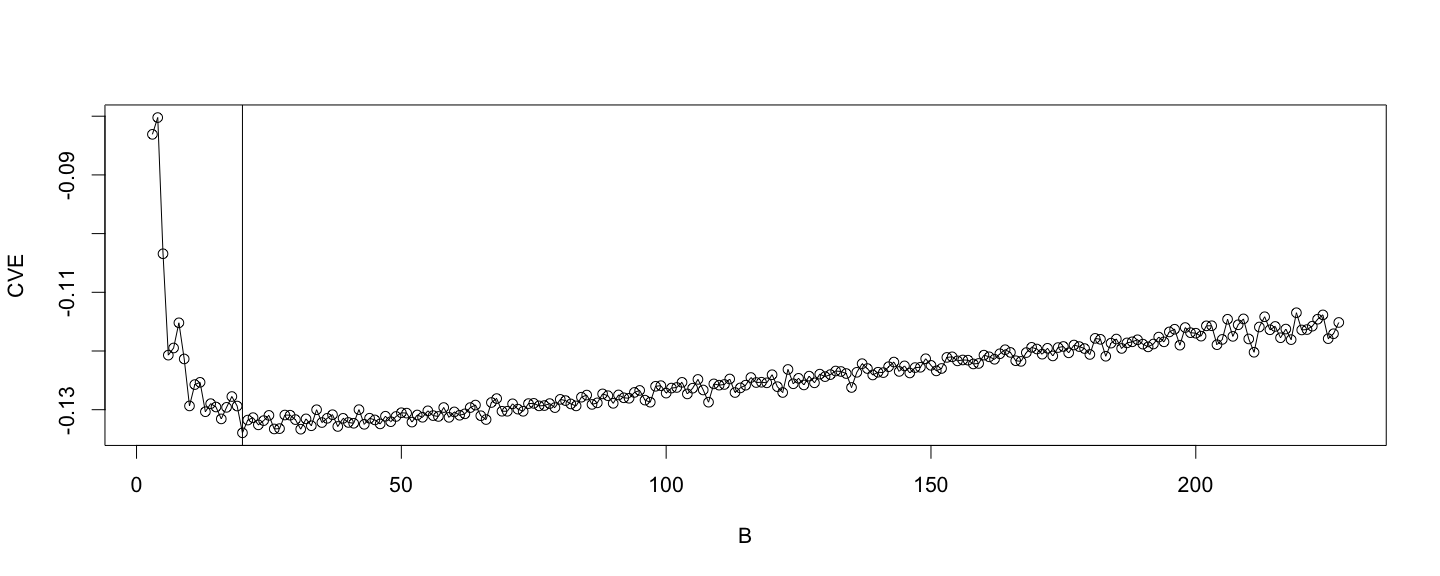
})

Cross validation: comparison with other "rules"

(nclass.cv <- with(ll, B[which.min(CVE)]))

[1] 20

nclass.Sturges(xx)

[1] 11

nclass.FD(xx)

[1] 12

nclass.scott(xx)

[1] 12

Cross validation: Resulting histogram

breaks <- seq(ll$range[1], ll$range[2], length.out = nclass.cv + 1)
hist(xx, breaks = breaks)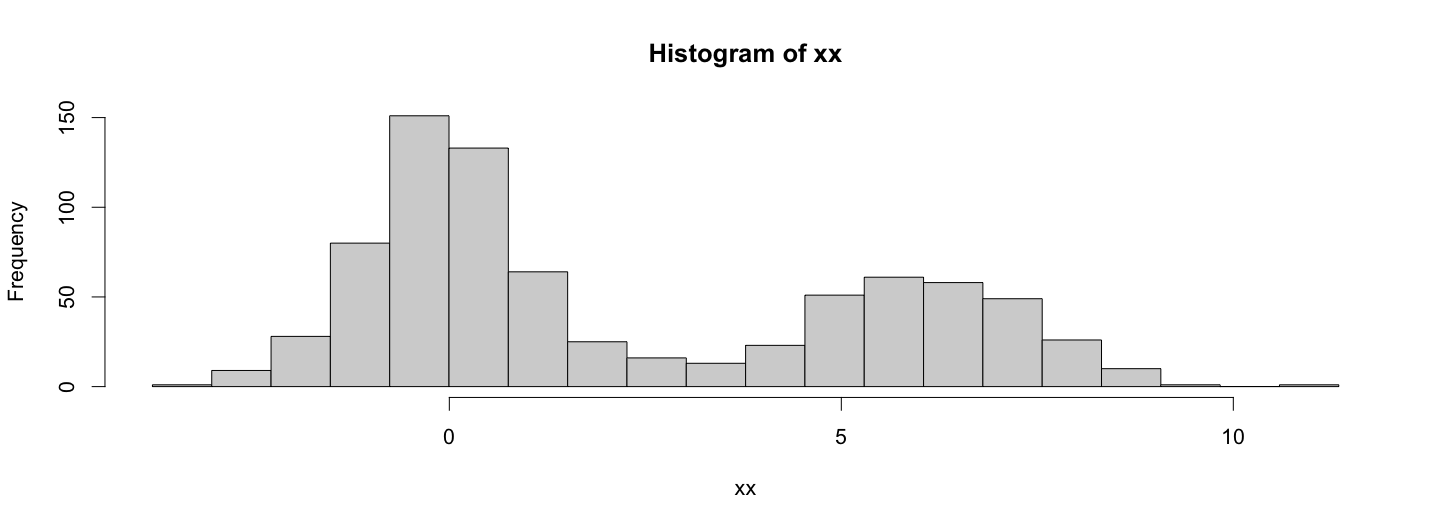

• For more interesting examples, see Gentleman and Ihaka, Lexical Scope and Statistical Computing

Related topic: non-standard evaluation

• Again, consider an expression that will cause an error when evaluated

rm(list = c("x", "y")) # remove x, y if defined earlier
plot(x, y, type = "l")

Error in plot(x, y, type = "l"): object 'x' not found

Quoted (unevaluated) expressions

• R can actually work with an expression without evaluating it

e <- quote(plot(x, y, type = "l"))
e

plot(x, y, type = "l")

e[[1]]

plot

e[[2]]

x

e[[3]]

y

Evaluating Quoted expressions

• A quoted expression can be evaluated using eval()

eval(e)

Error in plot(x, y, type = "l"): object 'x' not found

• Fails because current environment (.GlobalEnv) does not contain variables x and y

• But Recall: Environment e2 defined earlier contains

ls.str(e2)

x :  num [1:101] 0 0.0628 0.1257 0.1885 0.2513 ...
y :  num [1:101] 1 0.998 0.992 0.982 0.969 ...

Evaluating Quoted expressions

eval(e, envir = e2)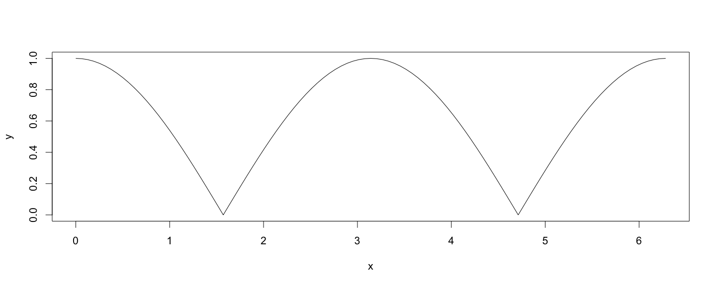

Can we re-implement the replicate() function?

• This is how functions like replicate() and with() work

my.replicate <- function(N, e)
{
    ans <- numeric(N)
    for (i in 1:N) ans[[i]] <- eval(e)
    ans
}

• But we have to be careful to use it

my.replicate(5, max(rnorm(10))) # not what we wanted

[1] 2.1574 2.1574 2.1574 2.1574 2.1574

my.replicate(5, quote(max(rnorm(10))))

[1] 0.5284321 0.6858938 1.3573033 0.8895072 1.6434051

Non-standard evaluation

• The substitute() trick: non-standard evaluation (using lazy argument evaluation)

my.replicate <- function(N, e)
{
    expr <- substitute(e) # avoids the need to quote()
    ans <- numeric(N)
    for (i in 1:N) ans[[i]] <- eval(expr)
    ans
}
str(x <- my.replicate(1000, max(rnorm(20))))

 num [1:1000] 1.648 2.524 1.636 1.346 0.729 ...

Lazy evaluation

• Lazy evaluation: function arguments are only evaluated when needed

set.seed(123)
rm(sqrt) # remove the sqrt() we defined earlier
chooseOne <- function(a, b, u = runif(1))
{
    if (u < 0.5) a else b
}

• Only one of a and b is evaluated in any particular execution

chooseOne(sqrt(2), sqrt(-2)) # no warning message

[1] 1.414214

chooseOne(sqrt(2), sqrt(-2)) # warning message

Warning in sqrt(-2): NaNs produced

[1] NaN

Further reading

? environment
? eval
? expression
? quote
? bquote
? substitute
? with

with.default

function (data, expr, ...) 
eval(substitute(expr), data, enclos = parent.frame())
<bytecode: 0x7f9061b19fb0>
<environment: namespace:base>

replicate

function (n, expr, simplify = "array") 
sapply(integer(n), eval.parent(substitute(function(...) expr)), 
    simplify = simplify)
<bytecode: 0x7f9061ac9e08>
<environment: namespace:base>