Using the rip.opencv package

Deepayan Sarkar and Kaustav Nandy

Introduction

The rip.opencv package provides access to selected routines in the OpenCV computer vision library. Rather than exposing OpenCV classes and methods directly through external pointers, the package uses standard R objects to represent corresponding OpenCV objects, and explicitly converts between the two forms as necessary. The idea behind this design is that most operations will be performed in R, and OpenCV is used to simply make an additional suite of operations available. Depending on use case, the opencv R package may be more useful for you, and a workflow mixing the two is facilitated by the image import / export functions in the respective packages.

As of now, the only OpenCV class that has an R analogue is cv::Mat, which can be used to represent an n-dimensional dense numerical single-channel or multi-channel array. It is used by OpenCV to store real or complex-valued vectors and matrices, grayscale or color images, and various other kinds of data. The R analogue of cv::Mat is an S3 class named "rip". Regardless of the number of channels, a "rip" object is stored as a matrix, with the number of channels recorded in an attribute along with the number of rows and columns.

A "rip" object can be created in R, most simply from a numeric (or complex) matrix.

suppressMessages(library(rip.opencv))
v <- as.rip(t(volcano), channel = 1)
v

[61 x 87] image with 1 channel(s)

class(v)

[1] "rip"    "matrix"

str(v)

 'rip' num [1:61, 1:87] 100 100 101 101 101 101 101 100 100 100 ...
 - attr(*, "cvdim")= Named num [1:3] 61 87 1
  ..- attr(*, "names")= chr [1:3] "nrow" "ncol" "nchannel"

An image() method for "rip" objects can be used to plot it (examples below).

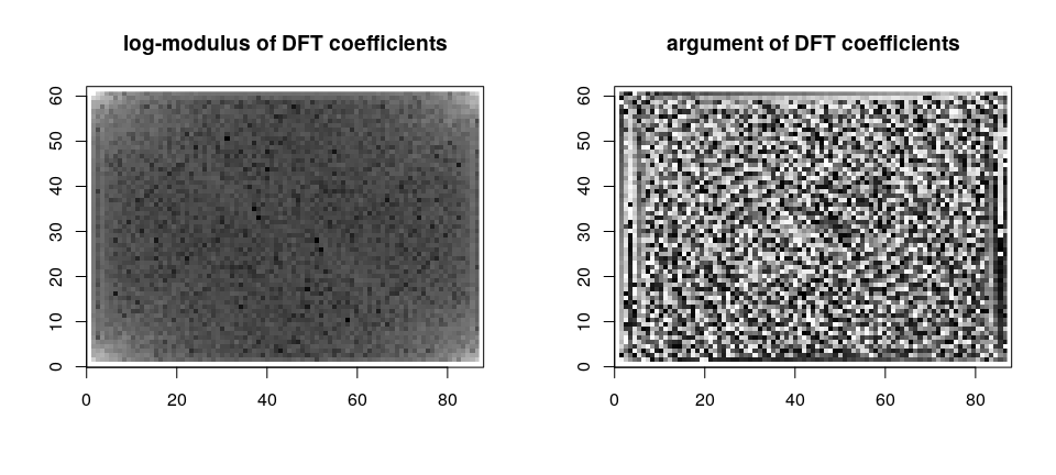
None of the above involves calling any OpenCV routines. Suppose we now want to use the OpenCV function cv::dft() to obtain a 2-D Discrete Fourier transform of v. This can be done using the high-level rip.dft() function as follows:

V <- rip.dft(v) # uses OpenCV function cv::dft()
V

[61 x 87] image with 1 channel(s)

str(V)

 'rip' cplx [1:61, 1:87] 690907+0i -53607-11919i -5986+182i ...
 - attr(*, "cvdim")= Named num [1:3] 61 87 1
  ..- attr(*, "names")= chr [1:3] "nrow" "ncol" "nchannel"

The return value is again an R matrix containing complex values wrapped in the "rip" class. We can use standard R functions for further processing.

par(mfrow = c(1, 2))
image(log(Mod(V)), main = "log-modulus of DFT coefficients")
image(Arg(V), main = "argument of DFT coefficients")

plot of chunk unnamed-chunk-3

Using the `"rip"` object for image manipulation

The most common use of a "rip" object is to represent a grayscale or color image. Grayscale images are essentially matrices, and their representation as a "rip" object is conceptually straightforward. Color images require multiple channels, and depending on the color space used, many different representations are possible. The "rip" class uses one particular representation, corresponding to the default cv::Mat representation for color images: For an n-channel image, rows correspond to rows of the image, and successive n-tuples of columns represent the n channels corresponding to each column of the the image (i.e., successive columns do not represent the same channel).

When plotting a color image using the image() function, it is assumed that the channels represent colors in the RGB color space and that columns are in the BGR ordering (this is the OpenCV default).

The rip.import() function uses the OpenCV function cv::imread() to read image data from a file.

if (!file.exists("Rlogo.png"))
    download.file("https://www.r-project.org/Rlogo.png", destfile = "Rlogo.png")
rlogo <- rip.import("Rlogo.png", type = "color")
rlogo

[155 x 200] image with 3 channel(s)

dim(rlogo)

[1] 155 600

str(rlogo)

 'rip' num [1:155, 1:600] 0 0 0 0 0 0 0 0 0 0 ...
 - attr(*, "cvdim")= Named num [1:3] 155 200 3
  ..- attr(*, "names")= chr [1:3] "nrow" "ncol" "nchannel"

Note that although the image is 155 x 200, the underlying representation is a 155 x 600 matrix. Extracting and manipulating individual channels in R is difficult with this representation. To facilitate such manipulation, the as.array() method can convert such an image into a 3-way array, with the third dimension representing channels in RGB order by default. By design, no array-like indexing operators have been defined for "rip" objects; vector and matrix-like indexing yields vectors and matrices, dropping the class attribute.

a <- as.array(rlogo) # add reverse.rgb = FALSE to retain column order
str(a)

 num [1:155, 1:200, 1:3] 0 0 0 0 0 0 0 0 0 0 ...

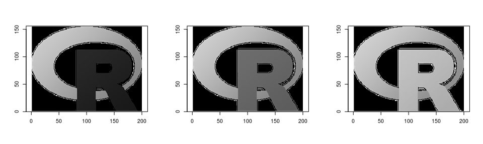
Individual channels can now be easily extracted.

par(mfrow = c(1,3))
image(as.rip(a[,,1]))
image(as.rip(a[,,2]))
image(as.rip(a[,,3]))

plot of chunk unnamed-chunk-6

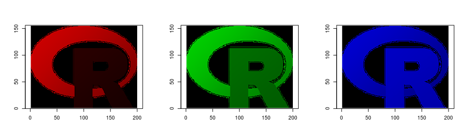
The as.rip() function can also handle 3-way arrays as input, interpreting it as a color image. This allows channels to be manipulated retaining the array structure before further processing.

par(mfrow = c(1,3))
red   <- a;   red[,,-1] <- 0; image(as.rip(red))
green <- a; green[,,-2] <- 0; image(as.rip(green))
blue  <- a;  blue[,,-3] <- 0; image(as.rip(blue))

plot of chunk unnamed-chunk-7

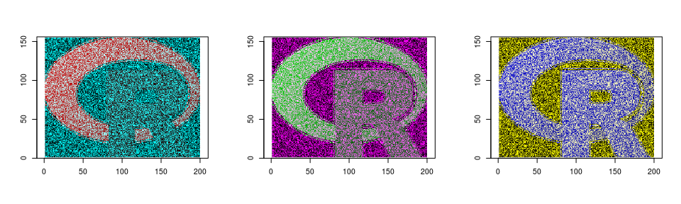
par(mfrow = c(1,3))
N <- prod(dim(a)[1:2])
  red[,,-1] <- runif(N, 0, 255); image(as.rip(red))
green[,,-2] <- runif(N, 0, 255); image(as.rip(green))
 blue[,,-3] <- runif(N, 0, 255); image(as.rip(blue))

plot of chunk unnamed-chunk-8

Similar methods are also available to convert to and from "raster" objects (in fact, this is how the image() methods works).

r <- as.raster(rlogo)
str(r)

 'raster' chr [1:155, 1:200] "#000000" "#000000" "#000000" "#000000" ...

identical(rlogo, as.rip(r))

[1] TRUE

Images imported using the png and jpeg packages can also be converted using suitable as.rip() methods.

require(png)

Loading required package: png

f <- system.file("img", "Rlogo.png", package="png")
img <- readPNG(f)
img.n <- readPNG(f, native = TRUE) # "nativeRaster" representation
str(img) # 4-way array

 num [1:76, 1:100, 1:4] 0 0 0 0 0 0 0 0 0 0 ...

str(img.n) # matrix of 32-bit unsigned integers

 'nativeRaster' int [1:76, 1:100] 0 0 0 0 0 0 0 0 0 0 ...
 - attr(*, "channels")= int 4

as.rip(img) # same as as.rip(img.n)

[76 x 100] image with 4 channel(s)

par(mfrow = c(1, 2))
image(as.rip(img))
image(as.rip(img.n))

plot of chunk unnamed-chunk-10

Modules

The rip.dft() and rip.import() functions are exceptions rather than the rule, in the sense that they are two of the very few high-level functions available in the rip.opencv package. Most functionality is instead exposed through low-level interfaces to selected OpenCV routines through Rcpp modules. These are not expected to be called directly by the end-user, and are rather meant to be used by other packages; careless use may lead to the R session crashing.

All modules in the package are available through the rip.cv variable, which is an environment containing named modules that group together similar functionality.

ls(rip.cv)

[1] "core"       "enums"      "feature"    "filter"     "imgproc"   
[6] "IO"         "photo"      "transforms"

The grouping is somewhat arbitrary and may change as the package evolves. For example, the IO module contains interfaces to the cv::imread() and cv::imwrite() functions, which are also exposed through the high-level functions rip.import() and rip.export(). However, one can also call a function in the module directly.

rip.cv$IO$imread

internal C++ function <0x5556b59546e0>
    docstring : Read image from file: type 0=grayscale, 1=color
    signature : Rcpp::Matrix<14, Rcpp::PreserveStorage> imread(std::vector<std::__cxx11::basic_string<char, std::char_traits<char>, std::allocator<char> >, std::allocator<std::__cxx11::basic_string<char, std::char_traits<char>, std::allocator<char> > > >, int)

We will use this function to read in a sample image. The result depends on a “read mode” flag, which is an integer code (the OpenCV documentation has details) that can be supplied explicitly. Some selected flags are available as named integer vectors in rip.cv$enums; these are not exhaustive but covers most common use cases. The following example reads in a color image in grayscale mode.

f <- system.file("sample/color.jpg", package = "rip.opencv", mustWork = TRUE)
(imreadModes <- rip.cv$enums$ImreadModes)

IMREAD_UNCHANGED IMREAD_GRAYSCALE     IMREAD_COLOR 
              -1                0                1 

(x <- rip.cv$IO$imread(f, imreadModes["IMREAD_GRAYSCALE"]))

[875 x 805] image with 1 channel(s)

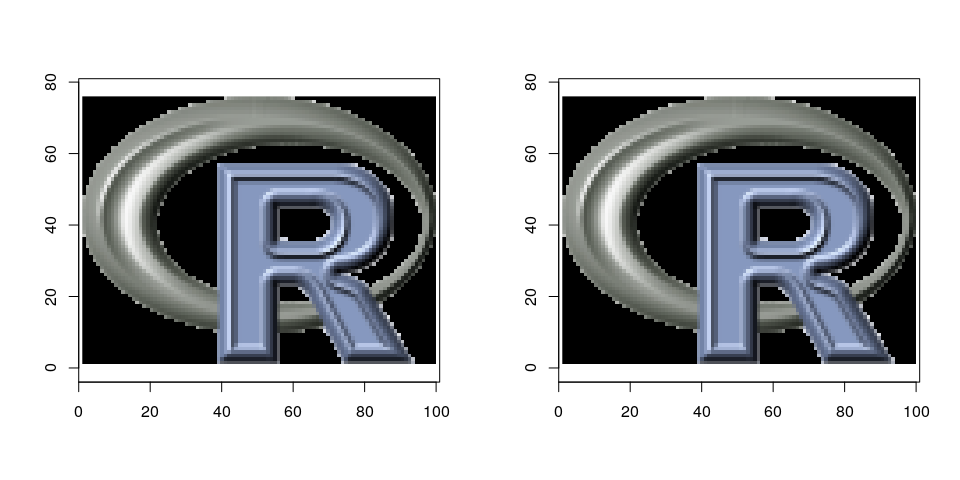
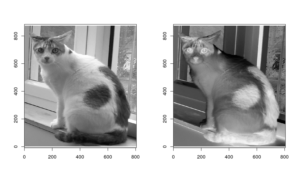
Once imported, the "rip" object can be manipulated as usual.

par(mfrow = c(1, 2))
image(x, rescale = FALSE)
image(255 - x, rescale = FALSE) # negative

plot of chunk unnamed-chunk-14

Example: convert color image to grayscale

We can of course read in the image in color mode as well.

(x <- rip.cv$IO$imread(f, imreadModes["IMREAD_COLOR"]))

[875 x 805] image with 3 channel(s)

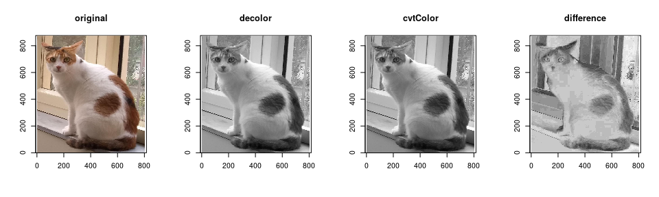
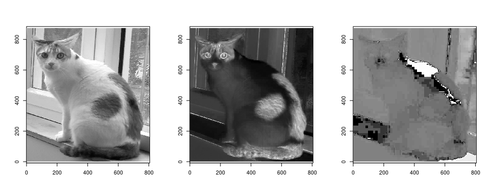
Suppose we now want to convert it into a grayscale image. One way to do so is to use the cv::decolor() function, which implements a contrast-preserving decolorization algorithm. Another alternative is to use the cv::cvtColor().

y1 <- rip.cv$photo$decolor(x)
convcodes <- rip.cv$enums$ColorConversionCodes
y2 <- rip.cv$imgproc$cvtColor(x, convcodes["COLOR_BGR2GRAY"])
range(y1 - y2)

[1] -6 13

par(mfrow = c(1, 4))
image(x, rescale = FALSE, main = "original")
image(y1, rescale = FALSE, main = "decolor")
image(y2, rescale = FALSE, main = "cvtColor")
image(y1 - y2, rescale = TRUE, main = "difference")

plot of chunk unnamed-chunk-16

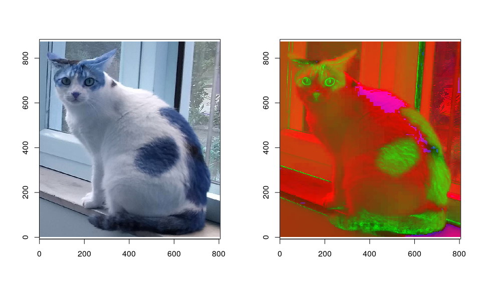
The cv::cvtColor() function is designed for more general color space conversion, and can be used, for example, to go from the default BGR channel ordering to RGB, or an entirely different colorspace such as HSV. The image() function always assumes BGR or grayscale, so it will be confused by such changes.

par(mfrow = c(1, 2))
x.rgb <- rip.cv$imgproc$cvtColor(x, convcodes["COLOR_BGR2RGB"])
x.hsv <- rip.cv$imgproc$cvtColor(x, convcodes["COLOR_BGR2HSV"])
image(x.rgb)
image(x.hsv)

plot of chunk unnamed-chunk-17

We can of course extract specific channels using as.array() from these objects; for example, the HSV channels can be plotted separately as follows.

a <- as.array(x.hsv)
par(mfrow = c(1, 3))
image(as.rip(a[,,1]))
image(as.rip(a[,,2]))
image(as.rip(log1p(a[,,3])))

plot of chunk unnamed-chunk-18

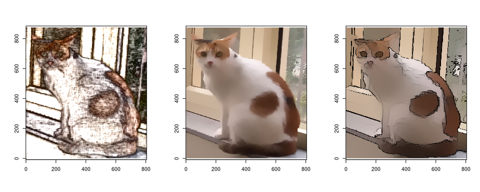
The following are more interesting examples of photographic image transformations.

par(mfrow = c(1, 3))
image(rip.cv$photo$pencilSketch(x, color = TRUE, 80, 0.1, 0.02), rescale = FALSE)
image(y <- rip.cv$photo$edgePreservingFilter(x, 2L, 60), rescale = FALSE)
image(rip.cv$photo$stylization(y, 60), rescale = FALSE)

plot of chunk unnamed-chunk-19

Other modules

A full list of currently available modules and the functions in them can be obtained as follows (FIXME: find better way).

do.call(rbind, lapply(ls(rip.cv), function(m) data.frame(Module = m, Function = .DollarNames(rip.cv[[m]], ""))))

       Module                      Function
      core                        PSNR( 
      core              copyMakeBorder( 
      core                        flip( 
      core                      rotate( 
     enums                   BorderTypes
     enums                      DftFlags
     enums            InterpolationFlags
     enums                   ImreadModes
     enums          ColorConversionCodes
    enums                          Misc
  feature                       Canny( 
  feature      cornerEigenValsAndVecs( 
  feature                cornerHarris( 
  feature           cornerMinEigenVal( 
   filter                GaussianBlur( 
   filter                      Scharr( 
   filter                       Sobel( 
   filter             bilateralFilter( 
   filter                        blur( 
   filter                   boxFilter( 
   filter                    filter2D( 
   filter             getDerivKernels( 
   filter              getGaborKernel( 
   filter           getGaussianKernel( 
   filter                  medianBlur( 
   filter                 sepFilter2D( 
  imgproc                    cvtColor( 
  imgproc                      dilate( 
  imgproc                equalizeHist( 
  imgproc                       erode( 
  imgproc               getRectSubPix( 
  imgproc         getRotationMatrix2D( 
  imgproc       getStructuringElement( 
  imgproc       invertAffineTransform( 
  imgproc               matchTemplate( 
  imgproc                     pyrDown( 
  imgproc       pyrMeanShiftFiltering( 
  imgproc                       pyrUp( 
  imgproc                      resize( 
  imgproc                  warpAffine( 
  imgproc             warpPerspective( 
       IO                      imread( 
       IO                     imwrite( 
       IO                      vfread( 
    photo                     decolor( 
    photo        edgePreservingFilter( 
    photo        fastNlMeansDenoising( 
    photo fastNlMeansDenoisingColored( 
    photo                     inpaint( 
    photo                pencilSketch( 
    photo                 stylization( 
transforms                         dft( 
transforms           getOptimalDFTSize( 
transforms                        idft( 
transforms                mulSpectrums( 

The choice of functions as well as their organization into modules are somewhat arbitrary, and details may change as the package evolves. Not all of these are well tested, and most are thin wrappers around OpenCV functions that take one or more cv::Mat objects as input and produce one as output. More routines may be added in future; an incomplete list of potential candidates are available here.

It is of course perfectly reasonable to want operations that combine multiple OpenCV functions, especially those that involve structures and classes more complicated than cv::Mat. Such functions (written in OpenCV) can also be wrapped, although there are few examples as of now. A very simple example is rip.cv$IO$vfread, which reads in a single frame from a video file.

High level wrappers

Apart from the modules discussed above, the package provides a few high level functions for common tasks that do more error checking and give a more R like interface. These include:

rip.import(), rip.export() for file import and export respectively,
rip.desaturate() for converting color images to grayscale, supporting several methods,
rip.pad() to add borders to a matrix with various kinds of border extrapolation,
rip.resize() for resizing matrices using various kinds of interpolation (including bicubic and bilinear),
rip.blur() for various kinds of blurring,
rip.flip() to reverse row and column order, and
rip.filter() for filtering and convolution.

In addition, the rip.dft() function, and its normalized version rip.ndft(), are designed to compute the 2-D DFT of a matrix and its inverse. These are particularly useful because they provide a non-trivial amount of sugar around cv::dft() in terms of handling complex values and combining various DFT flags. A related function rip.shift() shifts rows and columns by half, which is useful for changing DFT coefficients from a $[0, 2\pi]$ range to $[-\pi, \pi]$ and back.